


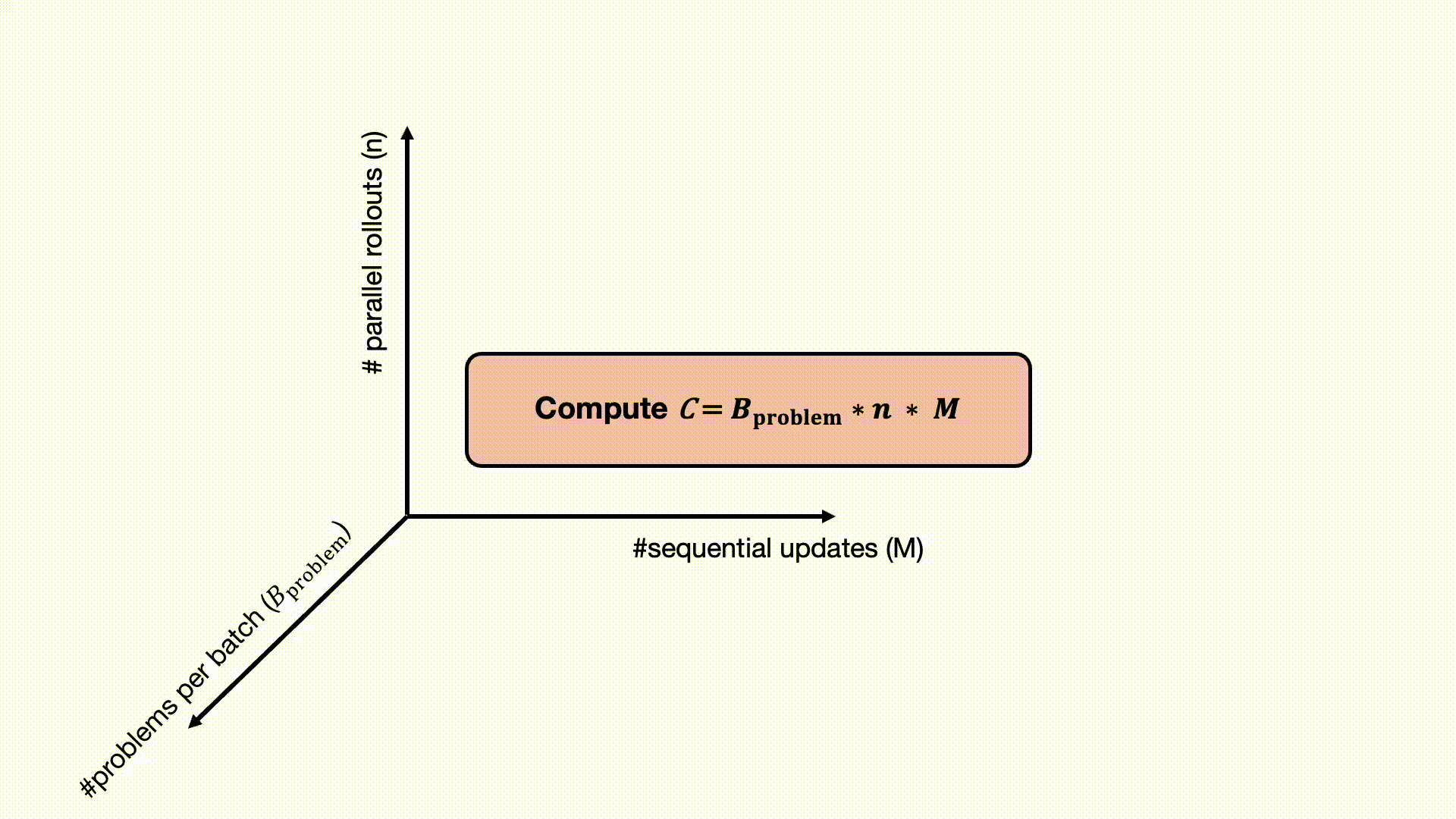
Figure 1: We study the compute-optimal RL for LLM along three axis: #parallel rollouts(), #problems per batch(), and #sequential iterations(), where total rollout compute . We find that (1) optimal parallel rollouts per problem () grows with compute budget (). (2) Easy and hard problems: similar scaling trends, but different mechanisms. (3) under fixed hardware constraints ( = × ), prioritize large (small ) at low compute budgets, but shift to large (small ) at high compute budgets to maximize performance (3) #problems per batch () has marginal impact on performance when kept in a moderate range.
A persistent blocker to scaling up reinforcement learning (RL) for LLMs is the absence of a concrete workflow: a recipe that tells practitioners what to scale in the recipe, how to scale it, and what outcomes of scaling one should expect. In many areas of modern-day AI, such workflows emerge from empirical scaling laws1 2 3: small-scale experiments reveal how performance should grow with compute, data, or model size. These laws inform compute allocation, models to use, and hyperparameter settings.
For RL, scaling laws remain far less understood compared to pre-training or supervised learning due to the interplay between data collection (exploration) and optimization (learning from data). Recent works have begun to sketch what these laws might look like in classical deep RL settings 4 5 6. But in the LLM setting, this line of work is still in its infancy. The most relevant prior results7 show that, under specific conditions (a particular problem mixture), reward curves in RL follow a clean sigmoidal shape when run for longer. Another prior work8 shows that RL training exhibits similar scaling behavior as pre-training in the model size, but ignores other hyperparameters. Simply fitting the shape of a learning curve or showing gains with larger models however does not answer one major question scaling laws intend to address: resource allocation to set up an RL run under the conditions that a downstream user faces. Given a base model, a problem set, and a total budget on compute, how should one spend this compute? If we had 10x more compute, how should that be spent? Which hyperparameters affect this resource allocation question the most and why? How does resource allocation change when the base model changes?
We have been working toward answering these questions. This article aims to frame the core scaling issues and provide practical guidance for allocating compute in on-policy RL for LLMs, with a particular focus on compute spent on on-policy sampling (rollouts). The resulting picture is nuanced: scaling behavior is governed not just by total compute, but by its interaction with the base model and the prompt distribution. Nevertheless, we find that predictable allocation rules for key hyperparameters emerge as a function of increasing sampling compute under a healthy (stable and scalable) recipe. Concretely, for on-policy RL algorithms that optimize policies using multiple parallel rollouts per sequential gradient step, we observe the following:
- Optimal parallel rollouts per problem () grows with sampling compute budget (). As the total sampling budget increases, the optimal grows following a predictable sigmoid. This indicates to maximize performance, practitioners should configure based on their the compute budget: allocating larger when given a higher compute budget; smaller when the compute budget is small.
- Easy and hard problems: similar scaling trends, but different mechanisms. While both easy and hard problem sets benefit from scaling , the underlying mechanisms are different. On easy problems, larger number of rollouts () primarily acts to sharpen the policy on already solvable problems, indicated by the improvements in the worst@k metric. In contrast, on hard problem sets, scaling is essential for expanding coverage (discovering rare successful trajectories), directly improving the best@k metric.
- The number of unique problems per batch () impacts easy and hard problem differently. We find that varying the number of unique problems per batch () yields negligible changes in validation reward, provided it is neither too small or too large, given a fixed number of parallel rollouts (). Thus, under fixed hardware constraints on total batch size (), this insensitivity dictates a dynamic allocation strategy: prioritize large (small ) at low compute budgets, but shift to large (small ) at high compute budgets to maximize performance. However, the trade-off on hard problems where reward is hard to obtain is more nuanced and may be hard to predict apriori.
- The scaling trend of parallel rollouts () generalizes across setups, while its saturation point is context-dependent. We find the benefits of scaling at higher compute hold across different base models and datasets, the specific value at which saturates is governed by three key interactions: a) Base model. Intrinsic model capacities dictate the sensitivity to interference and transfer across problems, shifting the effective range of before performance plateaus. b) Problem set size. Smaller datasets lower the saturation point due to early overfitting on easy problems, where validation reward degrades despite training reward gains, rendering very large values infeasible. c) Problem distribution. Harder problems saturate at lower values as they require a critical mass of sequential updates to make progress, effectively constraining the budget available for width. Furthermore, on skewed distributions, the scaling trend holds, while the optimal is heavily influenced by the specific metric one wishes to optimize (due to interference between easy and hard prompts).
Where RL Scaling Laws Come From (When They Exist), Conceptually
To begin, it helps to recall why scaling laws can be derived in supervised learning or pre-training, and what makes learning dynamics predictable in these settings. In supervised learning, the objective is typically cross entropy, which is smooth and optimized over a fixed data distribution. This results in relatively well-behaved optimization dynamics, where small parameter updates lead to small and predictable changes in the loss. Consequently, under well-chosen hyperparameters, which can often be identified through small-scale experiments, the training dynamics of supervised learning become predictable, allowing the loss to be modeled as a function of compute or data. The statistical structure of the data, such as the covariance spectrum, remains constant through training. A simple mental model would be that the decay of this spectrum9 governs the power law scaling behavior observed in practice. We emphasize that this perspective is an approximation rather than a formal proof, but it provides useful intuition for why scaling laws emerge in supervised learning. In RL, the challenge of deriving any scaling law is two fold:
- the expected-reward objective (unlike cross-entropy) behaves non-smoothly across training iterations which make small perturbations to the parameters
- the data distribution itself depends on the policy being optimized.
When training LLMs with a binary 0/1 reward, we observe that the first challenge of non-smooth rewards is relatively mild, and that it is indeed possible to predict the expected reward. However, we did also see in our early experiments that attempting to fit other performance metrics (e.g., pass@k or worst@k) that practitioners might care about poses predictability challenges due to objective shift. For this reason, rather than fitting performance directly, we fit compute-optimal hyperparameters as a function of resources.
The second challenge is more fundamental. In online, on-policy RL, the base policy and every policy update determines the distribution of future experience, which is non-stationary. This in turn alters the effective data covariance seen by the policy. As training progresses, both the policy parameters and the data distribution evolve together. This violates the stationary data assumption with a fixed covariance spectrum that underlies many of the standard intuitions for scaling laws in supervised learning, and therefore the usual recipes for deriving scaling laws (e.g., in pre-training) are not directly applicable in RL.
We therefore will first seek an RL recipe whose learning dynamics scale predictably with additional compute. In online RL, performance scaling is governed by two tightly coupled mechanisms: exploration, which determines what data is collected, and optimization, which determines what and how effectively the model learns from that data. These mechanisms are inherently in tension. Exploration favors sampling unlikely but potentially informative behaviors, while optimization pushes the policy toward responses that already achieve high reward. In LLM settings, exploratory responses are often extremely low probability under the current policy, and training on them can destabilize optimization10. A common symptom of this instability is pathological behavior in the entropy of the model’s next-token distribution, which may grow uncontrollably. As a result, naive RL recipes lead to instability when run on different prompt sets. To mitigate this, we design what we refer to as a “healthy” RL recipe, in which data collection (exploration) and optimization are coupled smoothly that behavior remains stable and scaling trends can be predicted. Concretely, this entails avoiding off-policy samples, and using entropy or KL regularization only when supported by the prompt set. As we show in later sections, such recipes exhibit stable entropy dynamics and enable performance to scale in a regular manner, thereby admitting meaningful scaling-law analysis.
Given this tight coupling between data collection and optimization, small changes in exploration can substantially alter the data the model trains on next, leading to qualitatively different learning dynamics. As a result, RL training behavior differs substantially between easy and hard problems. We further find that repeatedly updating on the same data leads to overfitting and causes the policy distribution to shift too rapidly, breaking predictability. This effect is consistent with our prior work6, which shows that clean scaling laws in RL emerge only when off-policy reuse is limited (i.e., a low updates-to-data ratio) and optimization remains stable. Motivated by these findings, we focus on on-policy RL in the remainder of this post, and analyze scaling mechanisms separately for easy and hard problem regimes.
Our Scaling Question: Compute-Optimal Sampling for LLM RL
Before we prescribe our healthy RL recipes or state our results, we first formally outline the key scaling setups that we operate in. Ultimately, scaling laws are useful because they help us decide how to allocate limited resources such as compute or data in order to achieve the best possible performance. Typically, these laws are obtained by running controlled small-scale experiments and extrapolating the observed trends. Therefore, it is helpful to begin with a basic question: what resources actually matter in LLM RL? In our setting, where RL is used to train a given base model on a fixed problem set, what are these resources?
In standard RL, two resources are crucial: compute, often measured in training FLOPs, and data, measured in the number of environment transitions collected online. In LLM RL, an environment naturally corresponds to a single prompt or problem, and as mentioned above, we assume access to a fixed set of such problems. When running RL post-training of a given base model on this fixed problem set, data is created entirely by spending compute on a given problem (prompt) set because every training rollout is obtained by rolling out the model (and problems are often negligibly-sized in comparison; though not always, e.g., in multi-turn settings, but we do only operate in a single-turn setting). This makes the distinction between compute and data less clear. Thus, for our study, we consider compute to be the only fundamental resource.
Given the primary resource of compute, it is natural to divide it into training compute and sampling compute. In LLM RL, sampling compute usually dominates the overall cost because every step of exploration requires generating multiple samples in an autoregressive manner. In addition, we typically train on all the data that is collected. Unless response lengths are scaled drastically, both training and inference compute scale (roughly) linearly with the number of tokens. This gives us a useful simplification for studying scaling. We can treat the sampling compute budget as the main quantity to allocate, since training compute grows in direct proportion to it, and focus on finding the most effective way to spend sampling compute. Before we go into our problem statement, we present some notation to simplify our discussion.
Notation and Definitions
We define the primary symbols and their relationships as follows:
- : sampling compute, measured as the number of rollouts. We use rollouts instead of tokens because the number of tokens generated per rollout is hard to predict ahead of time. Empirically, accounting for tokens yields the same scaling behavior in log-log space (see Appendix D).
- : the total number of gradient update iterations in training (often called “steps” in common open LLM-RL frameworks).
- : the rollout batch size per iteration, i.e., the total number of rollouts collected in one iteration.
The total rollout compute scales as:
can be further broken down into two components:
- : the number of unique problems in the rollout batch of each gradient step.
- : the number of rollouts sampled per problem (also referred to as the group size in GRPO11).
To sum up, rollout compute can be decomposed into three resources, that we can allocate:
Problem Statement
At a high level, our central scaling question is the following:
Given a base model and a problem set, how should we spend a fixed amount of sampling compute to maximize post-training performance?
This simple question abstracts all of the complexity of modern LLM RL. We make a simplifying assumption and assume that response length, on an average, is captured in the constants, we are now left to allocate sampling compute into . In principle, we could carry out our analysis accounting for the compute spent in terms of the total tokens sampled instead of the total rollouts. However, in our experiments we observed that although response length might vary across settings, these variations manifest primarily as a constant offset in log-log space, leaving the fundamental scaling trends intact (see Appendix D for a comparison between rollouts and tokens). Hence, our conclusions would be similar whether or not we accounted for the sequence length, and we chose to ignore it for simplicity. Our scaling study is based on one model and a problem set, so we do not count them as resources. Hence, our formal resource allocation question is given by:
Given a base model, a problem set, and a sampling budget , find the configurations of that attain the best possible performance under a target performance metric.
Ideally, as more sampling compute is provided, the optimal values of should be such that more compute translates to better performance. This means that the underlying recipe for which we prescribe values of should be such that it scales in an healthy manner as more sampling compute is allocated. RL runs with LLMs often destabilize or collapse with many optimization steps, and this means that we must first prescribe a scalable/healthy RL recipe before studying the above resource allocation question. We anchor our main experiments on Qwen2.5-7B-Instruct12 and leverage Qwen3-4B-Instruct13 and Llama3.1-8B-Instruct14 for extending our observations later.
What Constitutes a Healthy RL Recipe for a Given Base Model?
Now, we discuss several characteristics of an RL recipe that lead to healthy optimization behavior. From our experiments, we identify a few key factors that consistently govern whether optimization and exploration remain stable and scalable: (1) the difficulty distribution of the dataset, (2) the behavior of token entropy, and (3) the learning rate. These are not the only factors, in fact, we also observe that “staleness” (or how off-policy the generated rollouts are) also affects scaling and performance, but leave a discussion of it from the current blog post to focus on fully on-policy approaches.
Factor 1: Dataset Difficulty Distribution
The first factor that informs the health of an RL run is the composition of the problem set. Easy problems, where the base model can already sample multiple correct traces, tend to produce rapid entropy collapse15 of the model’s next token distribution. In contrast, making progress on very hard problems16, where the base model can hardly sample any correct trace, requires careful optimization that actively couples with exploration. In fact, we show below that running standard RL recipes from training on easy problems often results in rather unstable behavior when the problem set is too hard. Recent works show training on such problems requires algorithmic modifications to make very hard problems “appear” easy first (see our blog post16 and RL grokking17). This means that the difficulty of the problem set relative to the base model often very directly determines the knobs behind a healthy RL recipe.
A practical way to quantify this difficulty is to evaluate the base model’s performance on the problem set prior to training. In this blog, we use the Guru-Math18 dataset for its sizable, carefully curated math problem collection with verified answers, which allows us to perform controlled sampling. We first measure the problem difficulty by avg@16 (average accuracy over 16 trials obtained for a given problem) with the base model we use for RL training and then construct training problem sets by difficulty:
- Easy problem set: avg@16 in [0.3, 0.6] (6k samples), with a 300-sample in-domain validation set.
- Hard problem set: avg@16 in [0.0, 0.0625] (5k samples), with a 300-sample in-domain validation set.
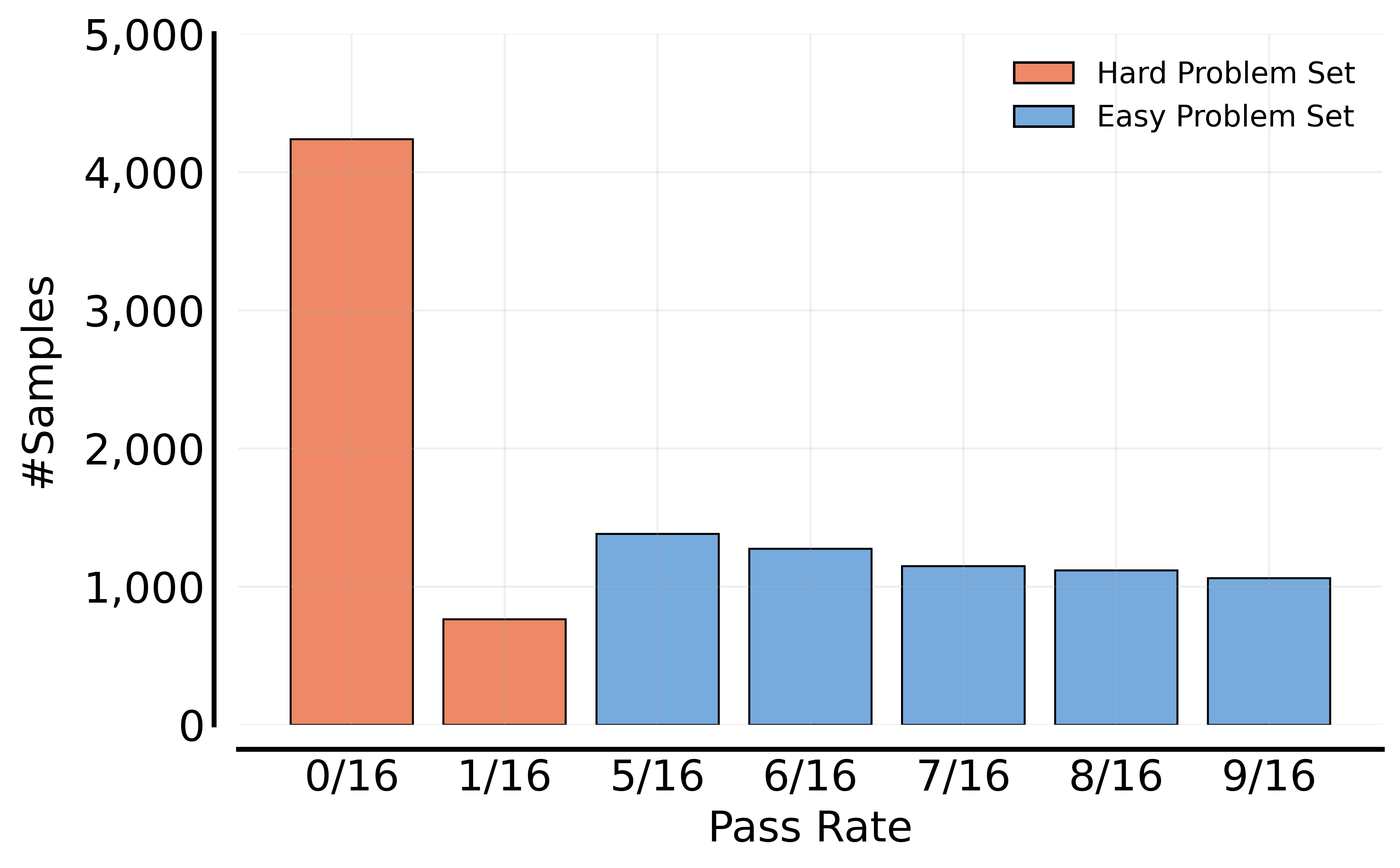
Figure 2: Distributions of problem difficulty for the Easy and Hard problem sets. Difficulty is quantified using avg@16, the average pass rate over 16 generations per problem.
Beyond these primary Easy and Hard sets for our experiments, we also curate a Heterogeneous set (mixing easy and hard set in different proportions) and an Extremely Hard (pass@128 = 0) for extending our observations. We default to utilizing the recipe for the Hard set on these problem sets as well. We discuss results on this set later in this post (see the section titled “The Bigger Picture”).
Factor 2: Entropy Control
The interaction between the problem distribution and the base model is very clearly reflected in token-level entropy and, also somewhat, in the KL divergence to the base model. While neither directly measures task performance, both serve as sensitive indicators of optimization health. When entropy or KL becomes too large or too small, learning can stall or become unstable. Intuitively, entropy controls how broadly the policy explores at the token level, while the KL divergence anchors the policy to the base model and limits excessive drift. The behavior of these quantities depends on problem difficulty. It is often a common practice to add an entropy regularizer for training. On easy problems, running RL without a sufficiently large entropy regularizer often leads to premature entropy collapse. However, on hard problems, running RL with an entropy regularizer alone often leads to an explosion in entropy and response length. A KL constraint by itself typically over-constrains exploration and is unnecessary in most regimes, indeed RL runs can work just as well without a KL constraint. However, on hard problems, where entropy can explode early in training, a KL anchor is effective at delaying or totally avoiding instability. For this reason, whenever we use an entropy loss, we pair it with a KL loss to provide a stabilizing anchor.
Prior work7 often employs a zero variance filtering (”zero-var filter” in Figure 3 below) mechanism when using rollout-based policy gradient methods such as GRPO, removing training prompts where all rollouts are either all incorrect or all correct. This filtering typically serves two purposes. First, it increases the effective batch size by keeping prompts that produce a non-zero policy gradient. Second, when entropy and KL regularizers are used, it prevents these regularizers from being applied on rollouts that do not contribute to an active policy gradient. The second mechanism is particularly important on hard problems, where RL optimization naturally pushes the policy toward higher entropy in order to discover rare positive trajectories that are unlikely to be produced by the base model but succeed. This increase in entropy is driven by the policy gradient19 itself and is often necessary for effective exploration.
Even with zero-variance filtering applied, problems in which rare positives are sampled can still experience an entropy explosion, since the resulting entropy or KL regularizers remain active. More concretely, our experiments (Figure 3) show that applying zero-variance filtering to the KL and entropy terms mitigates some of the most severe instabilities on hard problems. However, we find that it does not fully eliminate instability in all cases. Removing KL and entropy regularization entirely yields the most stable training dynamics. Thus, we adopt KL+entropy regularization on the Easy set, where entropy otherwise tends to collapse, and no KL or entropy regularization on the Hard set, to avoid instability.
Note that we adopt the configuration above: we apply KL+entropy on easy tasks and remove both on hard tasks, to prioritize training stability in our scaling study. Importantly, our scaling findings do not depend on this specific choice of regularization as long as training stability is maintained. For example, although the main scaling study employs KL and entropy regularization on the Easy set, we observe that the same scaling findings in the later section remain consistent under alternative setups on the Easy set, including both a “no KL / no entropy” configuration and a “KL + entropy with zero-variance filtering” configuration.
Experiment setup. We use Qwen2.5-7B-Instruct as the base model with a max output length of 8,192 tokens and employ the GRPO20 algorithm. We fix and . On both the Easy and Hard sets, we perform ablations over (1) the presence of KL and entropy regularization and (2) the application of the zero-variance filter, including variants where the filter is applied only to the KL and entropy loss terms.
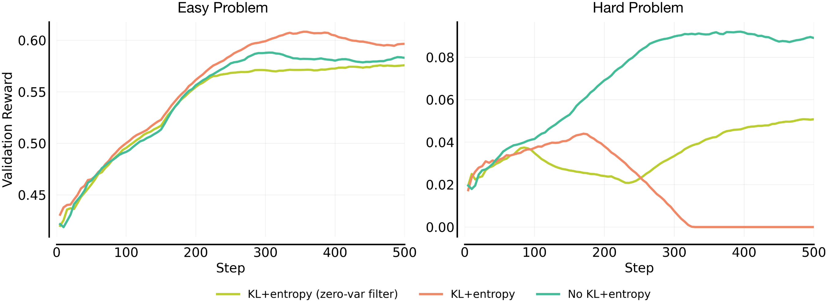
Figure 3: Ablations of KL+entropy and zero-var filter across the Easy and Hard problem set. On the Easy set, all configurations improve steadily, with standard “KL+entropy” achieving the highest reward (left). On the Hard set, while applying zero-variance filtering to the KL and entropy terms helps mitigate instability, disabling these regularizers entirely results in significantly more stable training (right).
Factor 3: Learning-Rate Scaling
Building on the perspective of stable entropy and KL dynamics, the learning rate (LR), denoted as , governs the magnitude of policy updates per unit of advantage. It is well-established that different model scales exhibit varying sensitivities to the learning rate2 3, and additionally the best learning rate depends on the batch size in supervised learning21 22 23. Since we vary the batch size in our experiments, establishing a robust baseline LR and a systematic scaling strategy is essential. To formalize this choice, we first identify a base learning rate anchor. We then study how different scaling rules perform as the batch size increases. Based on our experiments (Figure 4), we adopt as the anchor for a batch size of and utilize the square-root scaling rule with respect to .
Experiment setup. We conduct these experiments on the Easy set using the AdamW24 optimizer. The learning rate is linearly warmed up for 10 steps and then held constant for the remainder of training. We fix a baseline configuration with and run a grid search for a good base LR anchor. We then increase to and to and compare three scaling strategies:
- Constant LR: remains fixed regardless of changes in .
- Linear scaling: scales linearly with .
- Square-root scaling: scales proportionally to .
As shown in Figure 4 below, we observe that square-root scaling enables faster convergence while avoiding the instability seen in linear scaling. Although we ran this experiment on the easy problem set, we expect the same learning rate scaling strategy to apply across problem sets of varying difficulty. Conceptually, the way the learning rate should scale with batch size is governed by gradient variance and noise. While problem difficulty may change the optimal absolute learning rate, it should not fundamentally change the underlying scaling relationship as batch size increases.
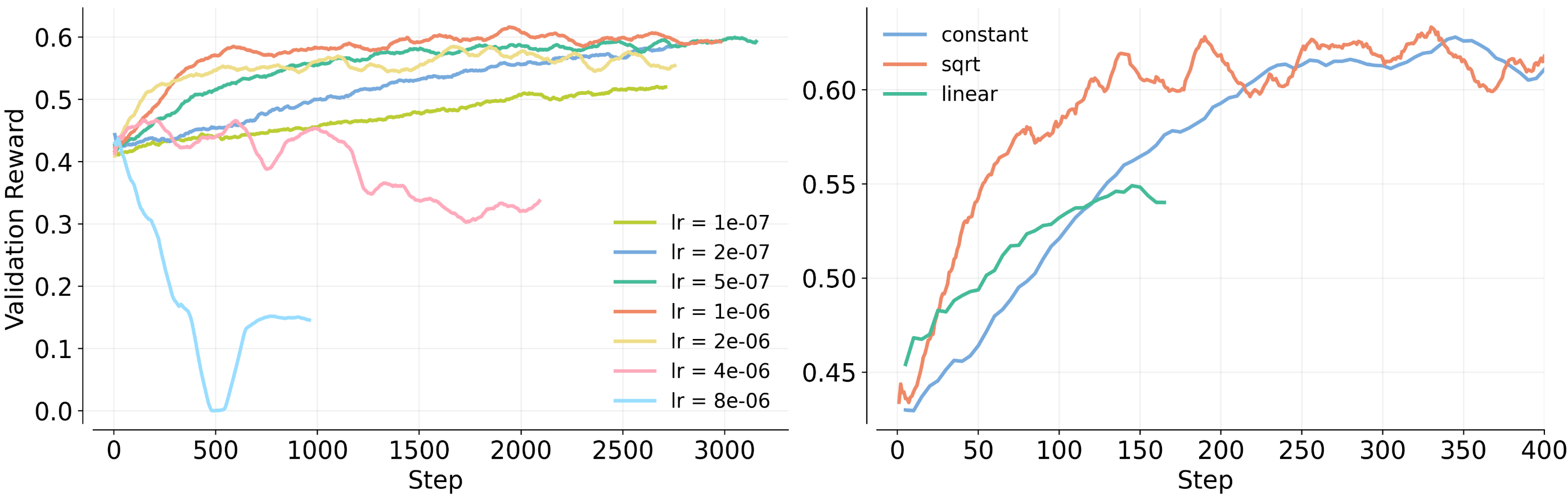
Figure 4: Base LR selection and scaling strategy validation. We sweep of the base learning rate at , and identify as the baselineLR (left).
We then compare LR scaling methods at a larger batch size (). Square-root scaling enables faster convergence without the instability observed in linear scaling, validating it as the robust choice for large-scale training (right).
Based on the ablations above, we use the following RL recipe for the coming scaling experiments.
| Distribution / Config | KL loss | Entropy loss | Zero-var filter | LR scaling |
|---|---|---|---|---|
| Easy | yes | yes | no | square root |
| Hard | no | no | no | square root |
- RL training exhibits distinct training behaviors depending on problem difficulty. We therefore explicitly curate and control for both Easy and Hard datasets to ensure the recipe is robust to different saturation points and exploration requirements. On heterogeneous datasets that we discuss later, we simply use the recipe corresponding to the Hard dataset to avoid instability.
- The necessity of regularization changes based on the difficulty level. Easy tasks benefit from KL divergence and entropy constraints to prevent premature collapse, whereas Hard tasks achieve peak performance when these loss functions are removed to enable stable training. Training on mixed datasets is most stable when no KL divergence or entropy are used.
- Learning rate should not be fixed as the total batch size changes, as in supervised learning. Of the schemes we compared, the square-root learning rate scaling strategy is the best.
Results: Compute-Optimal Allocation of Sampling Compute in LLM RL
We now turn to our central question: given a fixed sampling compute budget, how should we allocate it across the RL sampling knobs to maximize performance? Recall that the rollout compute scales . Our goal is not to tune a single best configuration for training, but to identify allocation workflows for distributing a fixed sampling budget across problems per batch and rollouts sampled for each problem in the batch. Across all experiments in this section, we sweep across a range of compute budgets . For a fixed compute budget , we evaluate multiple allocations and define the compute-optimal frontier as the highest IID validation set reward achievable using total compute . We get different plots on the frontier as we increase and sweep over values of .
Data analysis workflow. To make our scaling law prescriptions, we subsample the data from runs to only a smaller set of record-breaking points on a learning curve of reward (or any other performance metric) as a function of increasing compute. A record-breaking point is defined as the first point in a run that attains a higher validation reward relative to all previous points. For computing this higher reward, we first bucketize the reward into discrete bins and then pick the first points where the bucket increments.
More on the frontier definition
Formally, let denote all evaluated points, where is the compute spent so far and is validation reward obtained. The compute-optimal frontier is defined as . A configuration is record-breaking if . Any non record-breaking point is strictly dominated by a lower-compute alternative and therefore never attains for any . Consequently, the frontier induced by all runs is identical to the frontier induced by the record-breaking subset alone.
Restricting to record-breaking points is also more robust in practice. Non record-breaking configurations often reflect transient optimization instability, or stochastic variance in RL training, or sampling bias. We did attempt to fit a scaling curve over these points as well, and while it did not change the actual fitted curve, it made the fit more noisy. Therefore, we stick to fitting our curve over the record-breaking points only.
We then fit a monotonic function to the record-breaking points to obtain prescriptions for compute-optimal values of , , and . Because this pre-processing is order-preserving, this procedure does not introduce spurious non-monotonicity and yields the same frontier in practice as fitting over all points.
Unless otherwise stated, we use Qwen2.5-7B-Instruct as the base model with the max output length 8,192 and the healthy RL recipe from above. We use on-policy updates with an Adam optimizer, scaling the learning rate proportionally to , where the rollout batch size (base LR = 1e-6 at ); KL and entropy regularization are enabled on the Easy set and disabled on the Hard set (as discussed above); we fix the sampling temperature to 0.6 and to 1.0 for training and evaluation; we use GRPO to estimate advantages and truncated importance sampling (TIS25) to mitigate training-inference logit mismatch.
Experimental setup. We sweep over valid configurations from the Cartesian product , subject to the hardware constraint . We set for the Easy set and for the Hard set. The value of is smaller for the hard set to allow for more sequential iterations, within our allowed computational budget.
We concretely study compute-optimal allocation rules in three settings that allocate a subset of resources:
- vs (parallel rollouts vs sequential iterations)
- vs (parallel rollouts vs the number of problems in a batch)
- allocation across all resources.
Question 1: Trading Off Parallel Sampling with Sequential Iterations
We now examine compute allocation with the number of problems held constant, focusing on the trade-off between parallel samples and sequential iterations under a fixed compute budget.
Fitting workflow. We plot reward vs compute curves for each fixed and fit a monotonic sigmoid to summarize how the validation set reward (avg@4) scales with compute for that . As mentioned above, we then define the compute-optimal frontier as the upper envelope of these fitted curves (see Figure 5). Then, to indicate which lies on the frontier at each compute level, we color the frontier in Figure 5 by , which is the value of whose fitted compute–reward curve achieves the compute-optimal frontier up to . Finally, in Figure 6, we fit a log-log plot to show as a function of to summarize the empirical scaling behavior. We make four important observations in this setting.
1) The value of that lies on the compute-optimal frontier shifts systematically higher as the sampling compute increases (Figure 5). It is natural to expect larger values of to be generally favorable at higher compute budgets (echoing BroRL26), since increasing reduces noise in advantage estimates and lowers policy-gradient variance but eats up more sampling compute. Consistent with this, the frontier-attaining shifts to larger values as grows, and we observe the same trend in both the Easy and Hard problem sets. Smaller values of exhibit rapid initial gains but plateau at a relatively lower compute regime, whereas larger sustain improvement over a broader compute range (Figure 5). This behavior also suggests that parallel and sequential compute are not exactly interchangeable. Choosing so that we are able to perform a sufficient number of sequential updates is necessary to achieve strong performance.
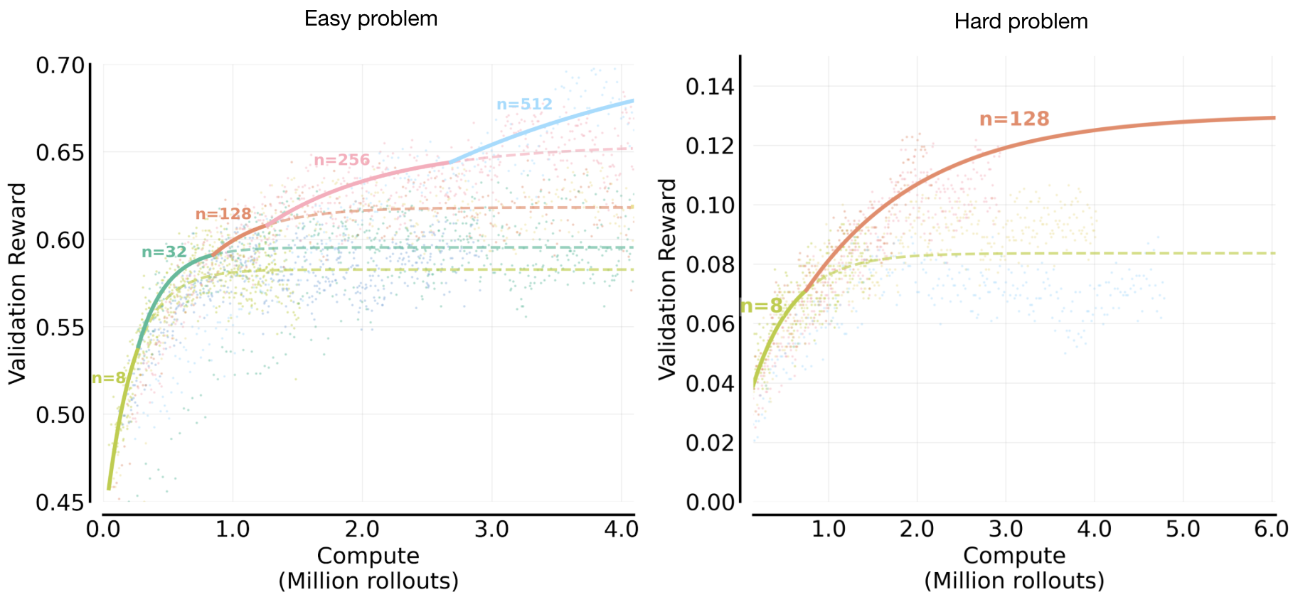
Figure 5: Validation reward frontier a function of compute , where the frontier is computed by maximizing over values of . The compute-optimal frontier shifts to larger with more , showing that more parallelism becomes optimal at higher budgets. For easy problems (left), small improves fast but plateaus; larger sustains gains and dominates at high compute. For the hard ones*(right)*, the same trend holds, but rewards are lower and saturate earlier, with the frontier reaching a smaller value than on the easy problems.
2) Compute-optimal values of are well-approximated by a sigmoid function of (Figure 6). We next seek to fit a functional relationship for the compute optimal value as a function of the available compute . A natural first step is to hypothesize an appropriate functional form. As shown in Figure 5, increasing admits larger compute optimal values of , and over a substantial range this relationship appears approximately linear on a log-log scale. The key question is whether this growth continues indefinitely or eventually saturates. Empirically, we observe a clear saturation in Figure 6. Even when evaluating rollout values up to , values significantly larger than the saturation point, they fail to extend the frontier, with continuing to dominate.
We argue that this behavior is expected for a fixed base model and a fixed problem set. To build intuition, it is helpful to view increasing as analogous to spending more compute per gradient step. In empirical risk minimization, increasing capacity alone does not reduce validation error beyond a certain point unless additional training data is available or the train-test gap is reduced. This principle also underlies pre-training scaling rules from Chinchilla27 that prescribe scaling both pre-training data and model capacity together. Perhaps most closely related to our RL training setup, our prior work28 on rejection fine-tuning shows that the optimal value of on the training set is often capped by an upper bound. Increasing alone cannot overcome limitations imposed by a fixed problem set for training or base model. As a result, the compute optimal value of must eventually saturate even for RL, which is precisely what we observe empirically. We empirically validate this hypothesis regarding model-data interaction in the later analysis section, where we demonstrate how the saturation point shifts given a different base model, problem set size, and distribution.
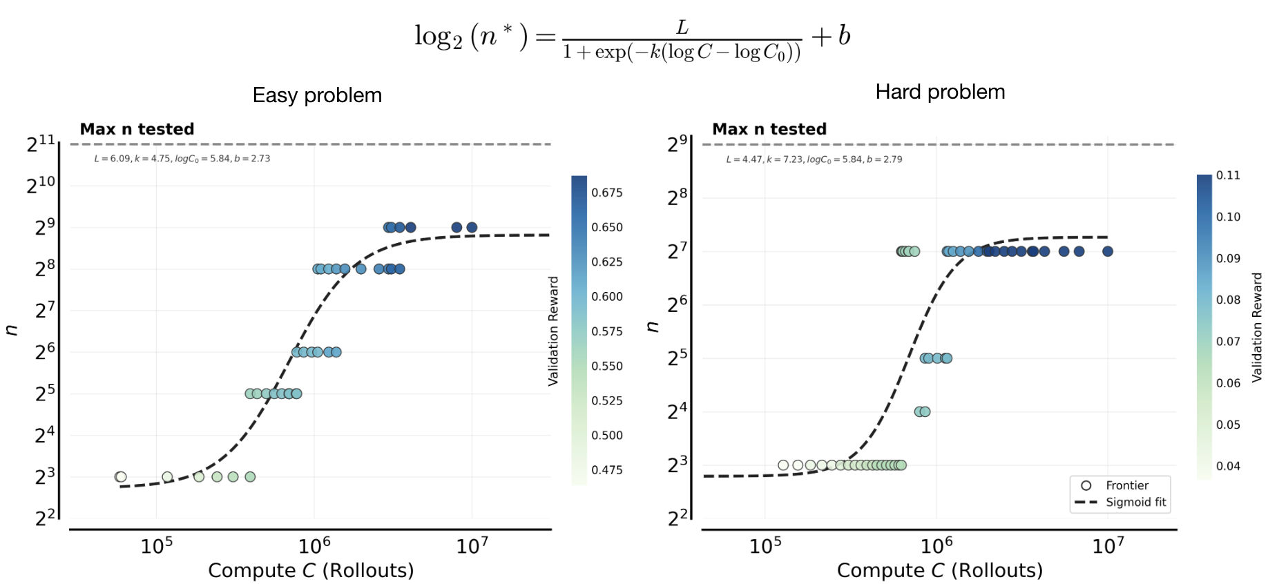
Figure 6: Compute-optimal scaling of the parallel compute (). The optimal value of rollouts shifts systematically higher as the total sampling compute increases. Points show a running-average estimate of the frontier-attaining at each compute budget (colored by reward), and the red curves fit a sigmoid parameterizing as a function of . For both the easy set (left) and hard set (right), rises from small to very large values as compute increases. On the hard set, the final value converges significantly below the maximal value of (), and this value is lower than the easy set.
3) Next, we find that the compute-optimal allocation trend remains consistent across difficulty levels, although we find harder sets prefer smaller values of (Figure 6). We find that the qualitative compute optimal allocation trend remains consistent across problem difficulty. On both easy and hard problem sets, the compute optimal value of increases with total compute before eventually plateauing. However, the plateau occurs at markedly smaller values of on harder problems. In particular, very large values of , such as , yield lower final performance on the hard set and do not lie on the compute optimal frontier. This suggests that task difficulty imposes an upper bound on how large can be used effectively. While it may seem intuitive that harder problems should benefit from larger due to increased sampling right away, we observe the opposite behavior in practice. On sufficiently hard problem sets, increasing allocates substantial compute to problems where the model receives little or no learning signal. In contrast, smaller values of focus optimization on the subset of prompts where nonzero signal is already present and meaningful improvement is possible. Therefore, if compute is bounded, it is better to use a smaller value of to increase the frequency of parameter updates (small , large , more epochs on the same subset of problems) that exploits reachable gains, rather than large parallel compute on problems that are persistently unsolved (large , small , fewer training epochs).
4) Implications on optimization dynamics on the easy and hard sets and the role of various performance metrics (Figure 7). We saw in point 3 above that a smaller value of was more preferable for optimizing validation average reward (avg@4 per problem), and we attributed this behavior to the underlying behavior of RL training (i.e., solving more problems vs producing more correct rollouts on the same problem). In this point, we aim to better understand this optimization dynamics and evaluate how changes if we were to change the target performance metric we study.
In particular, we consider two performance metrics: best@k (or pass@k) and worst@k. Recall the definitions:
- best@k: the proportion of problems where at least one generated response out of is correct. This measures the model's coverage over the validation problem set.
- worst@k: the proportion of problems where all generated responses are correct, also referred to as perfect solvability. This measures the robustness of the training procedure (i.e., the degree to which it can “sharpen” around the right solution).
Modulo compute-optimality, a larger value of coupled with as many sequential update steps as needed, should in principle, result in higher values for both best@k and worst@k on a training dataset. However, this is not quite the case when compute is bounded. We empirically identify the optimal values of for obtaining the highest best@k and worst@k scores on the validation set, across different values for the largest value of , and show this number in Figure 7 below. We choose , much smaller than any value of we study (), so that none of the trends in Figure 7 are “edge” cases or artifacts of empirical/fitting/workflow/statistical error. Perhaps surprisingly, we now see an interesting divergence in trends of compute-optimal that impacts the Easy and Hard sets differently.
- On the easy set, a larger is compute-optimal for worst@4 (sharpening) performance, whereas relatively smaller values of are compute-optimal for the best@4 performance. This means that a larger primarily improves by sharpening more on easy problems, while a smaller suffices to sample one correct rollout (expected since the set is easy).
- Conversely, for hard problems, a larger is more critical for pushing the best@4 (coverage) boundary, while a relatively smaller is compute-optimal for improving worst@4 (sharpening). However, there is a limit beyond which a larger does not improve coverage on new problems in a compute-optimal manner, as indicated by Figure 7 that optimal values here remain generally lower than on the easy set). On the Extremely Hard set consisting of all pass@128=0 problems (Appendix A, Figure 21 ), we see a clearer tradeoff of coverage and sharpening: while larger improves best@k, excessive degrades worst@k and lowers the average reward. Thus, if targeting average reward, the optimal on hard problems is the value that balances coverage and sharpening well.
The net effect of these distinct optimization dynamics is a similar trend of compute-optimal on the validation average reward (Figures 5 & 6), but these results imply that the target performance metric itself dictates the landscape of compute-optimal .
![**Figure 7: Different mechanisms of how $n$ values optimize best@4 vs. worst@4 on easy and hard problems.** For a given value of $B_\text{problem}$ on the x-axis, the $n$ values shown on the y-axis yield the highest validation reward under best@4 and worst@4 metrics. On the Easy set ***(left)***, the best value of $n$ for best@4 ::blue[(blue)]:: is smaller than the best value of $n$ for worst@4 (red), indicating that improving robustness ::red[(worst@4)]:: requires substantially more parallel rollouts compared to improving coverage. In contrast, this trend reverses on the Hard set: a larger $n$ is needed to improve best@4 in a compute-optimal manner, while the value of worst@4 saturates at smaller $n$ ***(right)***.](/assets/figures/sec3_q1_fixBprob_bestworstk.png)
Figure 7: Different mechanisms of how values optimize best@4 vs. worst@4 on easy and hard problems. For a given value of on the x-axis, the values shown on the y-axis yield the highest validation reward under best@4 and worst@4 metrics. On the Easy set (left), the best value of for best@4 (blue) is smaller than the best value of for worst@4 (red), indicating that improving robustness (worst@4) requires substantially more parallel rollouts compared to improving coverage.
In contrast, this trend reverses on the Hard set: a larger is needed to improve best@4 in a compute-optimal manner, while the value of worst@4 saturates at smaller (right).
- The compute-optimal frontier shifts systematically higher as the total sampling compute increases, which is well fit by a sigmoid curve.
- The trend remains consistent across training dataset difficulties.
- The source of gain from large shifts based on the training data difficulty: scaling improves sharpening (worst@4) on the Easy set, but expands coverage (best@4) on the Hard set.
- Depending upon the composition of the problem set, and how effectively can the base model learn on this set, we might see different underlying mechanisms for performance improvement. It is advisable to evaluate the mode of performance improvement for your base model on your prompt set, and accordingly use it to set as a function of the available .
Question 2: Bounded Parallel Batch Compute: Trading off with
Next, we study a different scaling setup, where wish to allocate a fixed total batch size into the number of prompts used and the number of rollouts per prompt used. This question is important in practical settings where hardware parallelism (e.g., number of GPUs or data-parallel workers) is fixed, and a practitioner needs to make this compute allocation. In such cases, is often chosen as the largest rollout batch size that saturates sampling throughput (”system batch size”). We experimented with for the Easy set under fixed to locate the upper and lower bounds for values of and that are effective.
We specify the number of sequential iterations a priori and seek allocations of and under a fixed total batch budget that maximize performance. We observe the following:
1) On the easy problems, allocate more parallel compute when sequential steps is large. In this regime, we examine the compute-optimal value of under a fixed total batch size (illustrated with only below), as varies. As shown in Figure 8, the optimal choice exhibits a sigmoidal dependence on . This behavior suggests that when more sequential update steps are available, it is generally preferable to allocate additional compute toward increasing , rather than increasing . In contrast, when is small, allocating batch size toward a larger is more effective, as it enables many more epochs of training on the same problems (Figure 9) within a given number of sequential updates.
On the Hard set, however, the scaling behavior is less consistent. The compute-optimal value exhibits a non-monotonic dependence on (see Appendix A, Figure 20), which implies a similarly irregular trend for the optimal . This is one of the main differences we see in scaling strategies across prompt sets of different difficulties. This happens because the Hard set behaves differently from the Easy set.
Across all settings, learning signal in RL can be increased through two complementary mechanisms: (i) sampling, by increasing to raise the probability of observing correct rollouts on a given problem, and (ii) coverage and generalization, by increasing so that policy updates are informed by a broader set of problems with at least some learning signal. On the Easy set, where the base model already produces correct rollouts reliably, the dominant bottleneck is sampling quality, making larger consistently preferable. On a harder problem set, we find that small values of remain ineffective at extracting a gradient signal when is small, even when it comes at the cost of training on a subset of problems in the Hard set. Next, when we increase , contrary to the easy problem setting, we find that increasing is now preferred as it avoids overfitting to the small training set of problems on which we got some signal initially. And then when we increase further we can now safely update on more problems without reducing for a higher , and the compute-optimal allocation once again demands a higher value of .
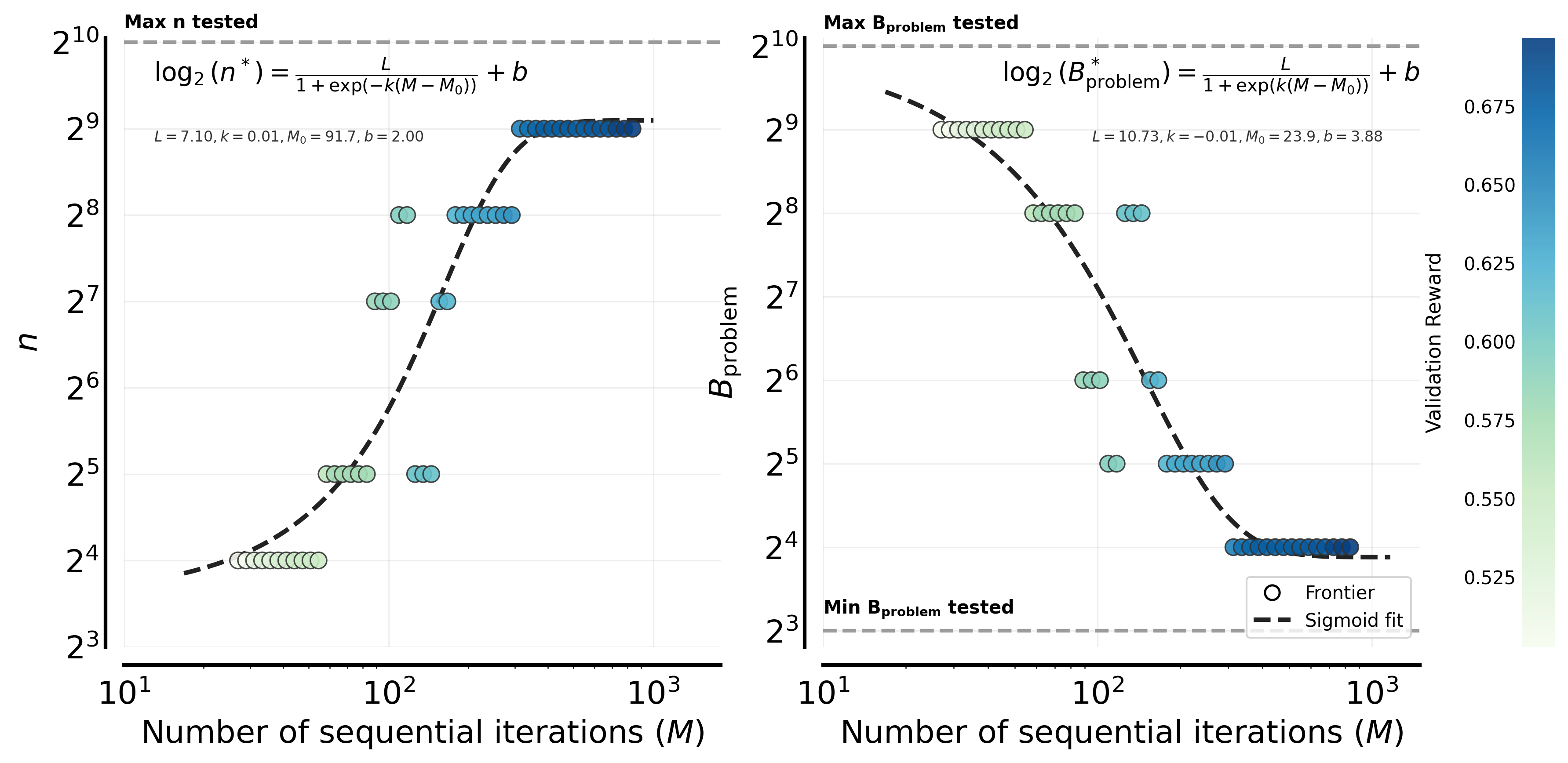
Figure 8: Compute-optimal allocation shifts from to under a fixed total batch size constraint () on easy problems.
We fix the total rollout budget per step () and sweep the number of sequential iterations (). A sigmoid relationship can explain the frontier of the optimal value of per problem. This curve indicates that increases with , a proxy of total compute given a fixed (left). The corresponding compute-optimal number of prompts decreases with the available sampling compute according to an (inverse) sigmoid (right). These indicate the strategic shift toward higher per-problem sampling at larger compute budgets.
Next, we ask what role does play? To answer this question, we study the effect of modifying for a fixed and the effect of modifying for a given and assess if performance is more sensitive to or . Our finding reveals that has minimal effect on validation performance.
2) has a marginal effect on validation performance when fixing . As shown in Figure 9 (left column), when fixing , varying on the Easy set provides little variance on validation reward. In contrast, increasing (fixing ) shows a strong correlation with improved validation scores, up to the saturation point discussed in Question 1. We also find a similar trend on the Hard problem set (Figure 9; right column). For the easy set, this explains the sigmoidal trend in Figure 8: since is the primary driver of performance and yields little difference, increasing is preferred for large and decreases in return (). However, though note that the variation in performance from and that from is overall smaller for the Hard set, which means that the optimal is more noisy; occasionally tilting the balance towards increasing to attain higher performance.
Overall though, we find that setting a large (up to the saturation point), with a moderate , is the most robust strategy. For example, in our experiments, we observed no significant threshold effects for between 32 and 1024 on the Easy set. However, on the Hard set or a skewed problem distribution, we speculate they may require a higher minimum for effective training. This behavior is intuitive. On a uniformly constructed Easy set (Figure 2), a relatively small but representative subset of problems already provides a good estimate of the underlying expectation. In contrast, for hard problems to the base model, training on a larger set of problems is necessary, since a small subset of problems that receive early learning signal can otherwise dominate through the course of training due to the “rich-gets-richer” dynamic of RL training. At the same time, the value of remains important. The resulting trade-off between problem coverage and per-problem leads to less predictable behavior on the Hard set (and explains the non-monotonic trends in setting and as shown in Appendix A Figure 20 and discussed above).
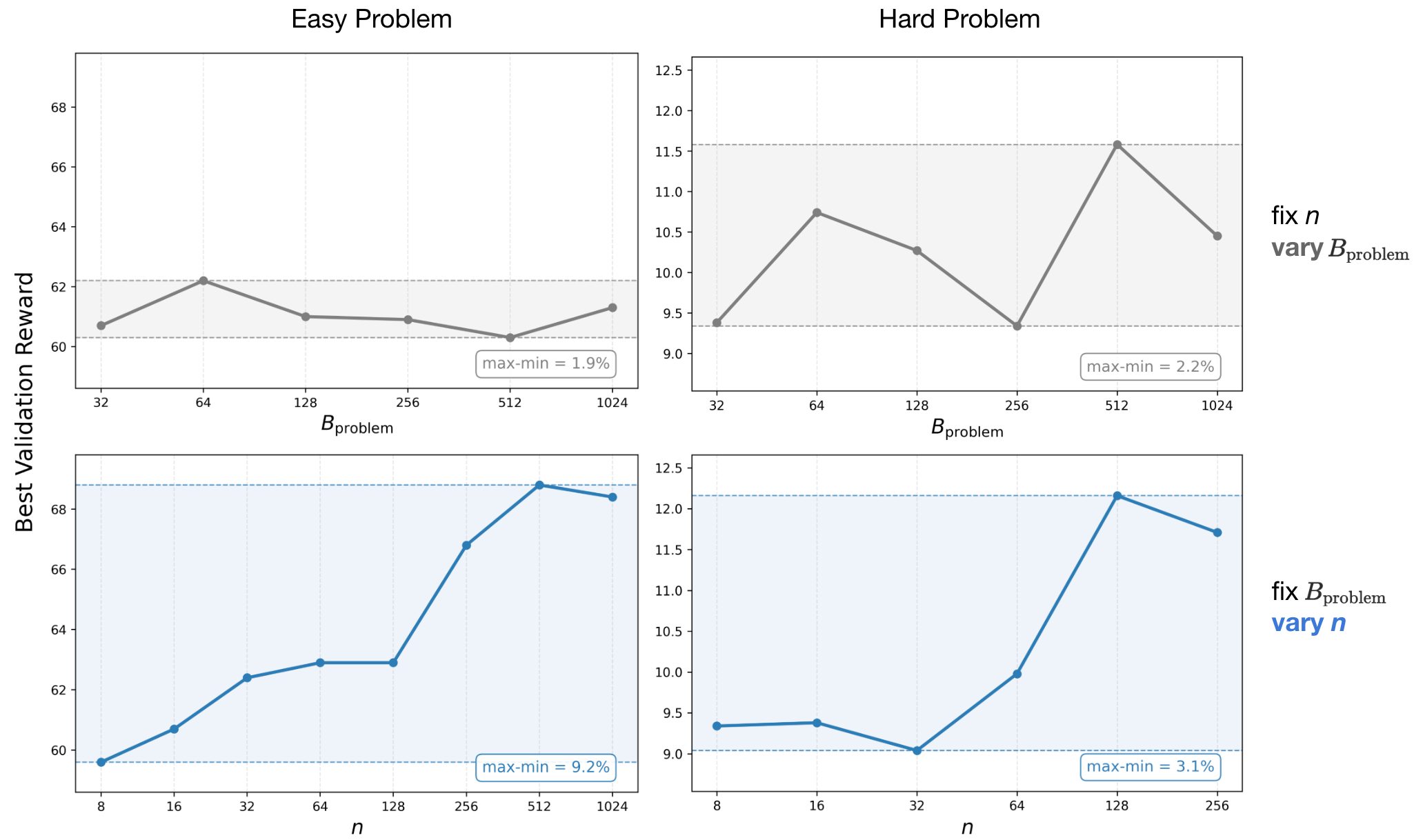
Figure 9: Sensitivity of validation reward to versus varying . Top Row: Varying with fixed . Bottom Row: Varying with fixed . Left (Easy): Validation reward is driven almost entirely by (9.2% variation; aligned with Question1 findings), while varying yields marginal impact (1.9% variation). Right (Hard): The trend is more nuanced. While remains important, the sensitivity to (2.2% variation) becomes significant relative to the sensitivity to (3.8% variation) given the inherently low reward regime of hard tasks. The fluctuating trend in the top-right plot suggests that selection introduces optimization differences on hard tasks, explaining the less predictable allocation trends when fixing on hard problems. That said, the trend of performance with varying values of for a given fixed (bottom row; Hard problems) is still monotonically increasing indicating predictability of the best value of .
- With a fixed total batch size , increasing compute favors allocating more rollouts () per problem and fewer problems per batch (). On the Easy set, this trend is clean following a sigmoid relationship, since large leads to rapid overfitting (as a result of multi-epoch training).
- On the Hard set, this trend is non-monotonic: increasing may be desirable at some intermediate values of . While scaling remains the more critical resource to allocate, must maintain a minimum threshold to avoid incomplete optimization.
- It is preferable to train on fewer problems with a sampling large budget if we are allowed training for multiple epochs on the same problem set. On the other hand, if multi-epoch training is not possible, then it might be preferable to include on more problems in a batch.
- The value of minimal allowed is larger for the Hard set compared to the Easy set, where and both lead to more comparable differences in performance.
Question 3: Putting It All Together
Finally, we relax all constraints and optimize jointly under a fixed compute budget. Consistent with our previous findings, the compute-optimal strategy is primarily defined by scaling . As shown in Figure 10 and 11, the optimal follows a sigmoidal trend as compute increases, regardless of problem difficulty. In this regime, acts as a stability constraint rather than a performance driver. We discussed in Question 2 that setting within a moderate range (e.g., 32 to 1024) only yields a small variation in performance. While we did not study massive values of where both and are large, and their interaction at large batch sizes is certainly important for future work to study, we do exhaustively sample values of and within the range we had access to. Our resulting practical recipe is simple: scale with compute according to the sigmoid, while keeping large enough to stabilize training.
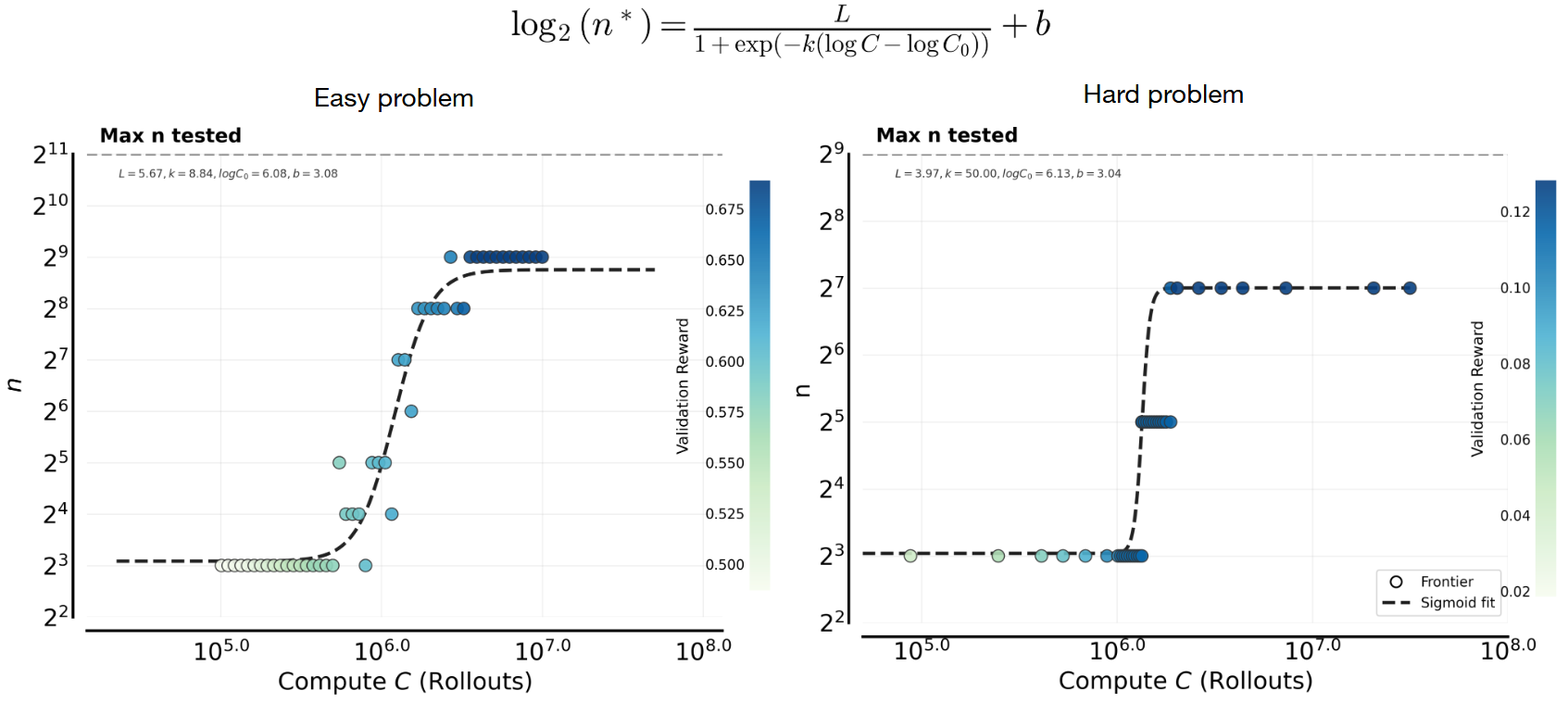
Figure 10: Compute-optimal parallel rollouts as a function of total compute , when , , and are all allowed to vary. We sweep hyperparameters () to find the global optimal configuration at each compute budget. The compute-optimal increases monotonically with compute, fit by a sigmoid function on both easy (left) and hard (right) problems.
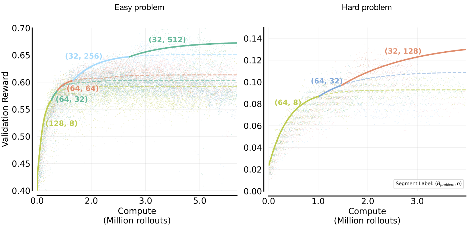
Figure 11: Compute-optimal frontiers sweeping () on easy and hard problems.
We annotate ( on the frontier as they are configurations before training and automatically scaled during training. Consistent with our earlier findings, the optimal shifts systematically higher as compute increases. While changes on frontiers, its impact on performance is marginal (as discussed in Question 2 Figure 9) and thus, unlike , the specific on the global frontier is more unpredicable.
- When jointly optimizing across all hyperparameters (), the compute-optimal value of still increases with , similar to the findings from Questions 1 & 2.
- Note the best total rollout size must generally increase as increases, though the compute-optimal value of can be roughly chosen to be a constant at all compute budgets.
- Our prescribed workflow suggests tuning first for a new model or new run, followed by allocating to a reasonable value and setting accordingly to the remaining compute. This provides the practical recommendation for users.
The Bigger Picture: Role of the Base Model and the Prompt Set
The recurring takeaway from the analyses above is that the compute-optimal number of rollouts, , increases with available sampling compute and eventually saturates as training becomes bottlenecked by other factors. While this conclusion is straightforward, a more interesting observation is that the same qualitative trend appears on both Easy and Hard sets. This naturally raises several questions: do we expect this behavior to exist on datasets of other difficulty levels? Does it extend beyond the single base model considered so far? More broadly, under what interactions between a base model and a prompt distribution should we expect this trend to generalize? In the remainder of this section, we address these questions using a combination of conceptual arguments and empirical evidence. We begin by studying an “idealized” setting of training on a single problem, examine when predictions from the one-prompt case break down, and finally analyze how interactions of the base model and prompt set deviations from this ideal behavior.
Base Case: Only One Training Problem
To build a conceptual model, let us study the simplest setting where we are provided with one single problem in the training set. We model this setting as a simple multi-armed bandit problem, where each arm represents one possible response to the problem. We assume training of a tabular softmax policy (i.e., softmax on independently represented logits denoting the response). Please see this for setup29.
Now let’s say that the base model attains an average pass@1 rate of on this prompt and say i.i.d. response samples drawn from the policy are used for training at one gradient step. First note that independent samples change exponentially: . Does change the policy gradient update on the problem in one update? Averaging over samples does not change the expected policy gradient direction: the expected update is identical to that obtained from a single sample. What it does change is the variance of the gradient estimate, which decreases by a factor . Prior work29 shows that, when using a single sample per update, tabular (stochastic) softmax policy gradient enjoys an rate on the policy suboptimality (i.e., bound on optimal performance - attained performance) after update steps. When independent samples are used by averaging over the policy gradient update, repeating the same analysis yields , where is a constant that does not depend on the variance of the policy gradient estimate. The constant in depends on variance in the policy gradient estimate and corresponds to the leading term (for reasonably small n).
With this guarantee, the convergence rate is still linear in , but the effect of stochasticity reduces drastically. For the term , and can be interchanged: one can reduce the error in this term by using a larger for a smaller . The other term depends only on , indicating that out of all compute allocation configurations in Question 1, for instance, one should prefer the configuration that makes more sequential updates as opposed to choosing a larger . However, this is not the case in practice.
Interference: Extending to Multiple Training Problems with Base Models
The theoretical argument above appears to contradict our empirical findings. While the theory suggests that sequential iterations (or ) take precedence over parallel rollouts , our results consistently show that is more critical. Why does this discrepancy arise? It cannot be explained by training on multiple problems alone, since the tabular analysis predicts similar convergence rates in that setting as well, provided learning rates are adjusted appropriately. We therefore attribute this gap to interference across problems30. When multiple problems are trained jointly, updates interfere, causing different problems to be learned at different rates and slowing overall progress relative to the single-problem setting. As training proceeds, the model’s ability to solve previously somewhat solvable problems degrades. In this regime, allocating compute toward larger values of is preferable to increasing , since higher number of rollouts promote more uniform updates across problems within each iteration. This shifts the compute-optimal balance toward parallel sampling rather than sequential optimization, mitigating interference and improving learning efficiency. The severity of interference also depends on the base model: some models admit representations where policy-gradient updates behave nearly tabular, while others exhibit strongly non-tabular interactions.
Evaluating interference. To understand the extent of interference, we visualize the evolution of the pass@1 distribution on the training set as a function of training steps. We observe that even on the Easy set (top row of Figure 12), where the initial pass@1 lies in the range , a non-trivial fraction of problems end training with no successful rollouts under both low (; Figure 12(a)) and high (; Figure 12(b)) rollout counts, when total compute is matched.
Under the same total compute budget (i.e., identical ), larger values of nevertheless lead to more uniform improvement across problems. In particular, the trained model’s pass@1 distribution in Figure 12(b) is closer to uniform, whereas the distribution for smaller in Figure 12(a) is more skewed, with mass concentrated on a subset of problems. This indicates that even on the Easy set, interference is present, and smaller results in less uniform updates across problems of varying difficulty, which mitigates some amount of interference: note that the proportion of problems with pass@1 = 0 is higher for a small in Figure 12 (a) at intermediate epochs compared to a large in Figure 12 (b).
A similar pattern emerges on the Hard set in the bottom row of Figure 12. When the base model initially fails on many problems, smaller concentrates updates on a limited subset of problems, rapidly pushing their pass@1 toward 1 while leaving others unsolved. This behavior is reflected in Figure 12(c), where the mass at pass@1 = 0 increases at intermediate training stages. In contrast, larger produces a more even distribution of probability mass across pass@1 values (Figure 12(d)), reducing the fraction of zero-pass problems and improving coverage. That said, both of these distributions are farther from the uniform distribution in absolute terms. This aligns with our earlier findings that, on hard problems, larger prioritizes expanding problem coverage rather than sharpening performance on already-solvable tasks.
Compute-optimal scaling generalizes for different base models. As shown in Figure 13, larger values consistently outperform the baseline () at high compute budgets for both Qwen3-4B-Instruct and Llama 3.1-8B-Instruct on their own easy (0.3-0.6 init pass rate) and hard (0 init pass rate) problems. However, the values of are specifically model dependent, and largely depend on the interaction between the base model and the problem set. We also observed that the validation reward for both models ceases to increase or degrades at on both Qwen3 and Llama3.1 on easy problems. This saturation in validation performance occurs while the training reward continues to rise. We attribute this divergence to the train-test gap (overfitting), that we discuss in the next section.
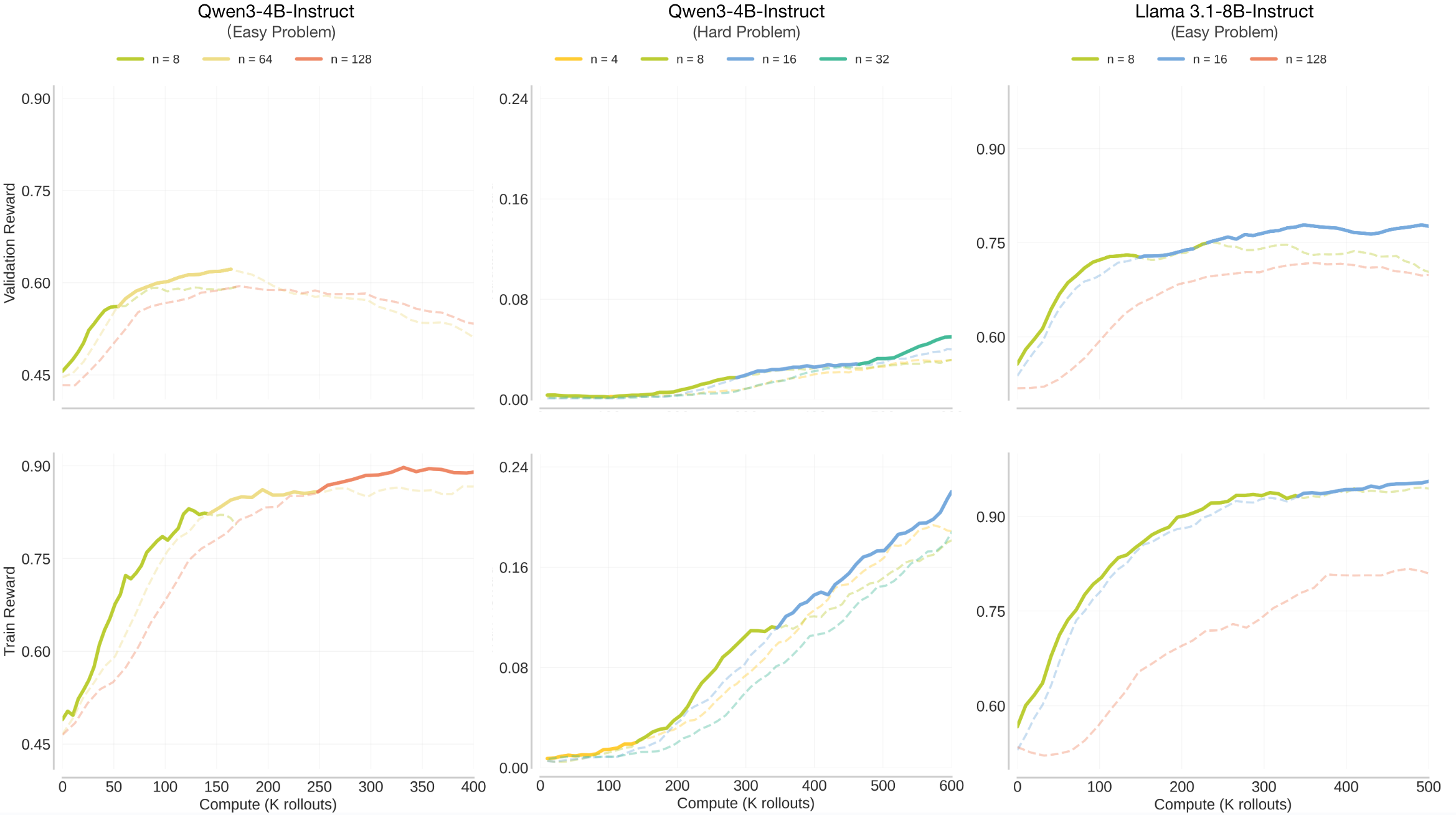
Figure 13: Generalization of compute-optimal scaling trends to other base models. We experiment with Qwen3-4B-Instruct and Llama 3.1-8B-Instruct on their own easy (0.3-0.6 pass rate) and hard problems (0 pass rate) with varying values. (1) We see that increasing improves performance at high compute across different models and difficulties. Specifically, the optimal outperforms baselines in all cases: Qwen3-Easy peaks at (left), Qwen3-Hard continues improving at (middle), and Llama-Easy peaks at (right). (2) The optimal saturates at lower values here (e.g., ) compared to the main experiments ( on easy and on hard).
This divergence suggests the train-test gap (overfitting) also affects the specific saturation point for each model-dataset combination. We dicusss the train-test gap in the next section.
A mental model of interference. From the above experiments, it is clear that perhaps a natural choice to model inference is through the distribution of across prompts. In fact, this distribution is a sufficient statistic in the tabular regime and also underlies inference-time scaling laws31 that relate at a population level to the distribution. However, in RL the model also learns from the rollouts it produces, and the pass@1 under the base model no longer fully characterizes training dynamics. This is because updates across multiple problems introduce interference, which inference-only scaling does not face. A useful mental model is that interference is minimized and updates are closer to the tabular setting when learning happens in a fashion that is roughly distributed uniformly across prompts. From this perspective, changes in the distribution over training can act as a diagnostic for interference. When the distribution improves approximately uniformly at all values of pass@1, then interference is relatively controlled; when improvements are highly uneven, stronger interference effects are present and we might observe a rich-gets-richer phenomenon. For instance, we observed interference on the Hard set, where there is fast improvement on a narrow subset of problems, and no improvement on the others (i.e., a large chunk of problems simply remain at a pass@1 value < 0.1). This notion of interference also manifests as distinct underlying mechanisms of reward improvement (coverage vs sharpening) in Question 1. Despite these differences, both problem sets ultimately exhibit the same scaling law for allocating compute.
Train-Test Gap
Our scaling results are reported on validation metrics, even though optimization dynamics are primarily driven by the training set composition. As a result, the emergence of scaling laws on the validation set depends on sustained transfer of performance from the training to the test set, which is not guaranteed. For instance, when the prompt set is too small, training may overfit prematurely within a fixed number of gradient steps. In such cases, larger values of may no longer appear compute-optimal at higher compute budgets, simply because additional training beyond some number of training steps fails to improve test-set performance (see Figure 14 as an example, where is never compute-optimal).
When overfitting dominates, scaling laws may only hold for certain ranges of hyperparameters that avoid the overfitting regime, but naively plotting scaling trends using our workflow above will result in incorrect conclusions. To illustrate this, we run training with different prompt set sizes, including sets substantially smaller than the default size of 6,000 problems used above. We observe that the compute-optimal values of cap out at much smaller levels when the prompt set is smaller. This behavior is expected, as validation performance begins to degrade with additional training compute in the small-prompt regime due to overfitting, meaning that there is no way for larger values to achieve the frontier. As discussed above, this also justifies the sigmoid shape of the hypothesized relationship between and in Figure 6.
Technically, we can also plot compute-optimal scaling laws for training performance instead of validation in the hope that compute-optimal hyperparameter configurations for best training rewards also results in best validation performance. We find evidence to the contrary as in many cases. Training runs with smaller values of (keeping fixed) result in better training rewards for the same amount of total training compute spent (see Figure 14). While this result appears contradictory at first, it is perhaps expected as training reward (in our logging scheme) logs rewards on samples that were used for training: hence, logging statistics on this set results in a natural bias. More mechanistically, on the training set: 1) RL runs with smaller values of are able to epoch faster on the training problems for the same amount of sampling compute as runs with larger values of ; and 2) when we run RL with small values of then we are able to improve training performance quickly on easy problems without making any progress on the hard ones, which means that the total training performance is dominated by only one set of the data (easy problems), which rightly does not reflect in good validation performance.
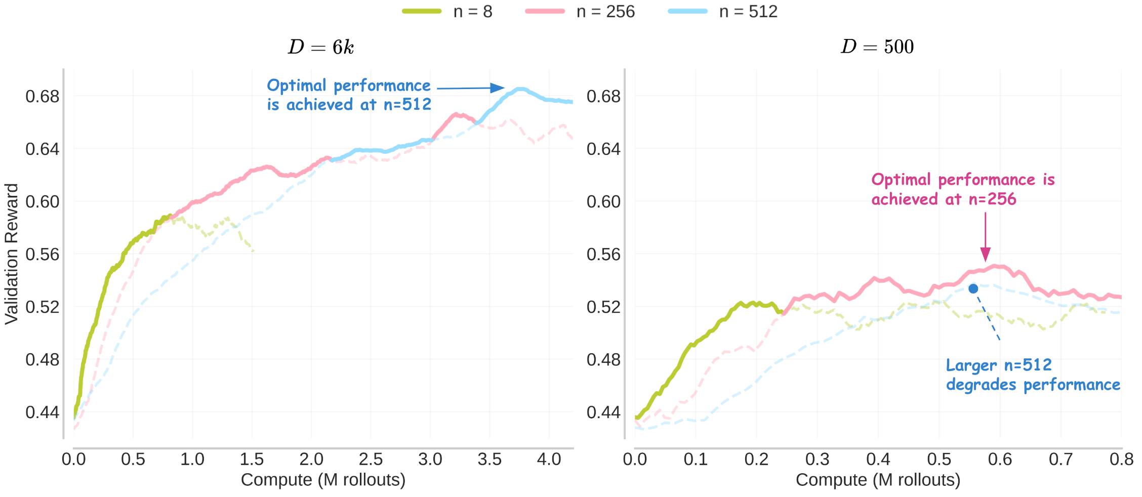
Figure 14: Impact of data size () on compute-optimal frontiers for Qwen2.5-7B-Instruct (easy set). With a larger dataset (), we continues to improve with more parallel rollouts (; left). With a smaller dataset (), performance peaks at , and a larger leads to degradation ().
Dataset Skew: Extension to Other Data Compositions
Finally, we train on several Heterogeneous mixtures of Easy and Hard problems (Figure 15), as well as on an “extra hard” set consisting of problems on which the base model attains an empirical of . These mixtures induce different degrees of dataset skew, which we expect to affect the rate at which improves during training (a smaller is likely to now improve more on easier problems in the subset resulting in more interference, while a larger should somewhat alleviate this issue). Despite this variation, Figure 15 reveals a consistent crossover trend: beyond a dataset-dependent compute threshold, larger values of outperform smaller ones across most validation sets. On particularly hard validation sets, larger often dominates almost entirely, or the range of compute over which smaller is optimal shrinks substantially. This behavior aligns with our findings from Question 1 and suggests that the rate of improvement controls both the width of the compute range over which a given is optimal and the minimum compute-optimal value of . Crucially, our central finding remains unchanged: larger compute budgets consistently support larger compute-optimal values of , even across highly skewed dataset mixtures.32
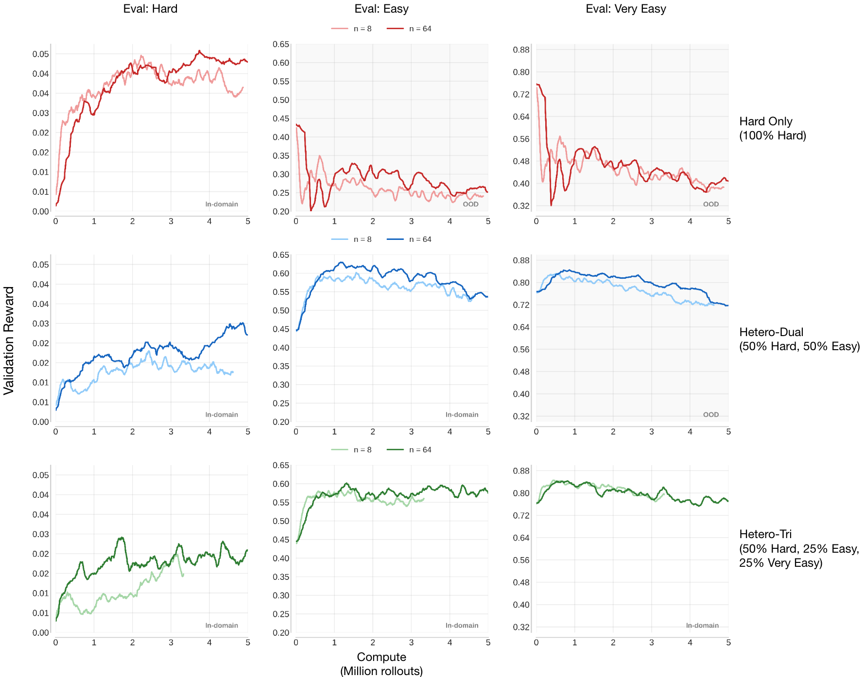
Figure 15: Results across difficulty levels for small () and large () budgets under different training data distributions (each with 5K total samples) using Qwen2.5-7B-Instruct. Data definitions: Hard (pass@128=0), Easy (pass@128 ), and Very Easy (pass@128 ). Training settings: Row 1: Hard Only (100% Hard); Row 2: Heterogeneous-Dual Mix (50% Hard, 50% Easy); Row 3: Heterogeneous-Tri Mix (50% Hard, 25% Easy, 25% Very Easy; the J-shaped distribution recommended in Polaris). On each data distribution, we observe a consistent trend that larger performs better at higher compute in in-domain evaluations, except for the very easy eval (Column 3). This task is likely so easy that added sequential or parallel compute does not make much difference in learning. Putting it all together, we see that training on all hard problems causes significant catastrophic forgetting on (very) easy problems, where the model could have decent pass rates, likely due to large distribution shift. When mixing easy problems in training, the catastrophic forgetting is largely mitigated on both easy and very easy problems, in exchange for a slight drop (~2%) on hard problems. A notable phenomenon is that mixing very easy problems (Row 3) doesn’t even help the in-domain very easy evaluation set, and degrades both easy and hard performance (compare with Row 2). These indicate: (1) if the focus is only on improving hard problem performance, it helps to train on all hard data; (2) otherwise, mixing easy data largely helps maintain the model’s capability, but very easy data are not useful.
- Interference: While sequential computation is more preferred in a tabular setting, interference across problems tilts the balance in favor of parallel computation; such that both and should be scaled as the available compute increases.
- Train-test gap and overfitting: The size of the training problem set manifests as a train–test gap: when the training set is small, validation performance saturates early. This leads to lower saturation values for and , and correspondingly higher optimal values of .
- Scaling rules transfer across data compositions: Although different base models exhibit different levels of interference on different problem sets, we observe similar scaling rules for how compute should be partitioned into parallel rollouts although for different underlying mechanisms. That said data compositions do affect the range of compute-optimal values of .
Discussion, Summary, and Future Work
A central takeaway from this work is that healthy RL recipes are inherently dependent on the prompt distribution and the behavior of RL training depends on the interaction between the base model and the prompt set, and that this dependence manifests directly in how optimal hyperparameters scale with compute. The same algorithm can exhibit qualitatively different scaling behavior on easy versus hard problem sets. On easier problems, increasing parallel rollout compute primarily improves sharpening and robustness, whereas on harder problems the dominant effect is expanded coverage. While trends in compute-optimal hyperparameters are often consistent when measured using average reward, they can diverge substantially under alternative metrics such as best@k and worst@k. This sensitivity to both data difficulty and evaluation metric highlights a key departure from supervised learning, where scaling behavior is typically more uniform once the model size is fixed. In RL, scaling laws are therefore inherently more nuanced, reflecting the coupled effects of optimization dynamics, exploration, task structure, and evaluation criteria. This study provides, perhaps the first, concrete framework for identifying and reasoning about these trends with base models and prompt sets, and empirically illustrates them across several regimes.
Our analysis also surfaces an important open challenge for future work: interference across problems. In an idealized single-problem setting, one might expect clean exponential improvements with increasing sampling compute. In practice, however, RL is performed over mixtures of problems, where progress on some tasks can interfere with learning on others. This population-level interference alters both the coefficients and effective hyperparameter values in observed scaling laws.
A promising direction is to identify sufficient statistics early in training that capture the degree of interference across problems, enabling more accurate predictions of how additional compute will translate into subsequent learning progress. We believe that tracking changes in the pass@1 distribution over the course of training provides a natural starting point for studying interference. Developing such models would be a critical step toward predictive scaling laws for RL on heterogeneous data mixtures. Mathematically, this points toward approximate closed-form rules for compute-optimal hyperparameters that generalize across base models and prompt distributions by estimating a small number of statistics that summarize the pass@1 landscape and incorporating them into scaling-law fits. This remains an interesting direction for future work.
Acknowledgements
We thank Oleg Rybkin, Apurva Gandhi, Charlie Snell, Matthew Yang, Rishabh Agarwal, Sang Michael Xie, Junlong Li, and Zora Wang for their thoughtful feedback on the blog. We also thank Chengyu Dong, Mikhail Yurochkin, Rupesh Srivastava, Joel Hestness, and Gavia Gray for early discussions on RL scaling in LLM. We also gratefully acknowledge the Orchard cluster at the FLAME center of CMU for providing some computational resources.
Appendices
A. Additional compute-optimal results
In the main results, we show one fixed value for for brevity. Figures 16 and 17 demonstrate that the scaling trend described in the main text, where larger compute budgets favor increased parallel rollouts (), holds across different fixed values of . While it appears that larger settings saturate at lower values (e.g., at ), this might be attributable to the total batch size constraint () in the sweep experiments. The precise interaction between and the saturation point of remains an open question for future investigation.
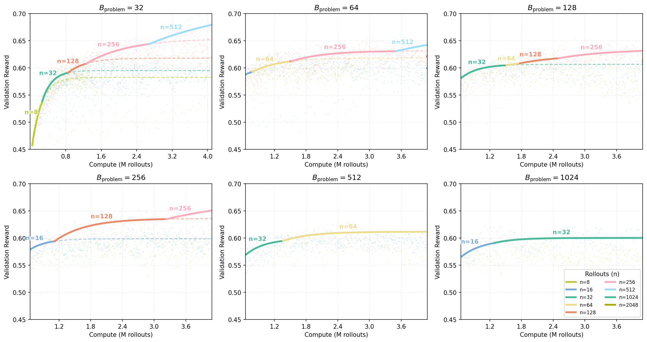
Figure 16: Compute-optimal frontiers across varying problem batch sizes () on the Easy set. Each subplot fixed and sweeps .
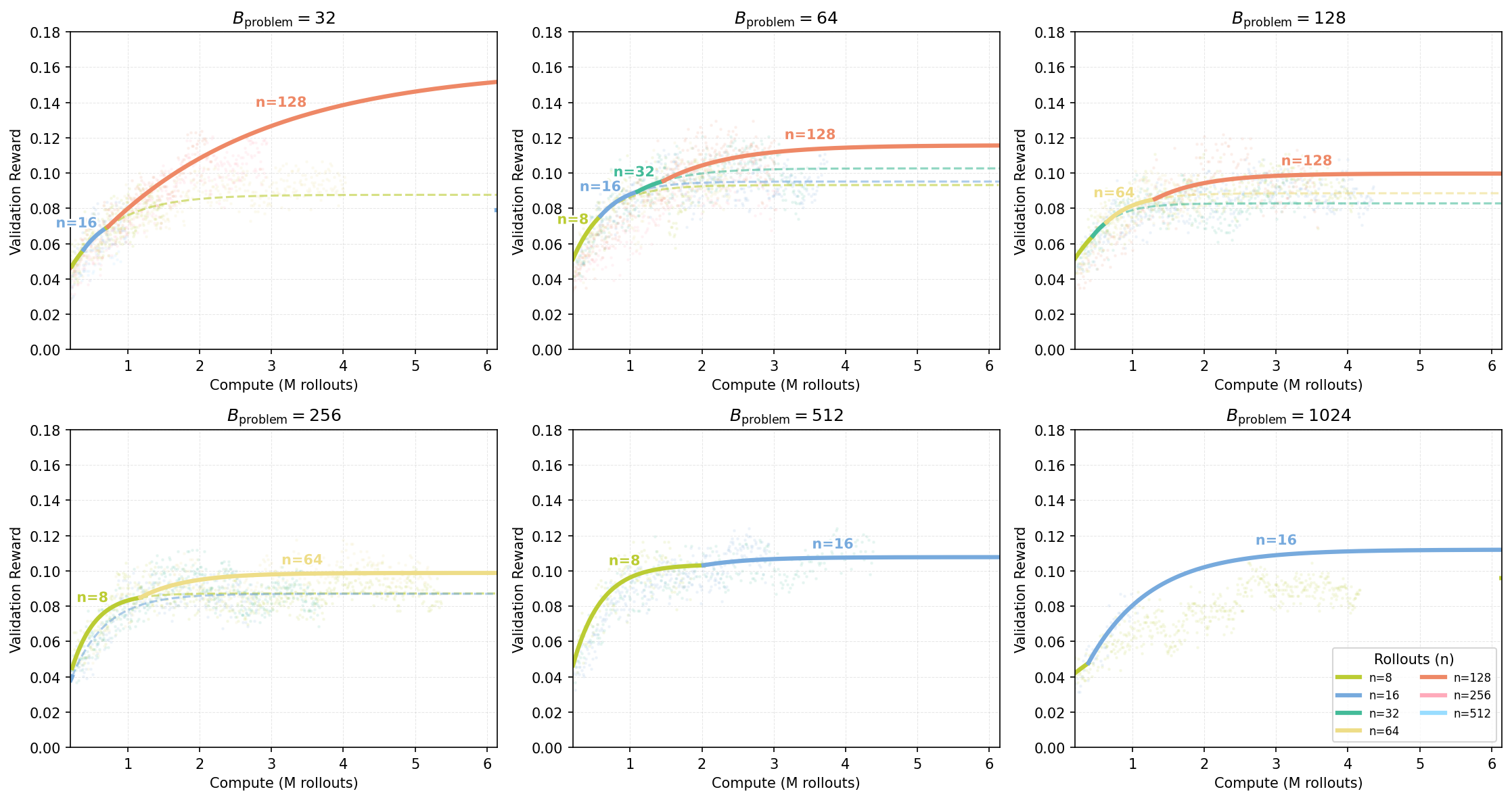
Figure 17: Compute-optimal frontiers across varying problem batch sizes () on the Hard set. Each subplot fixed and sweeps .
Figure 18 and 19 provide additional compute-optimal frontiers under different fixed values of on the Easy and Hard splits. Consistent with Section 3.2, higher sampling budgets increasingly favor larger , indicating that allocating more parallel rollouts per problem is a robust strategy across dataset difficulty and batch-size settings.
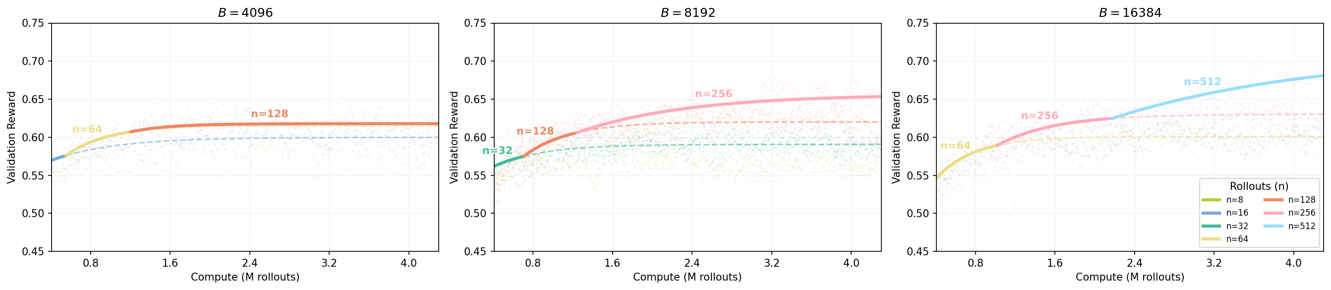
Figure 18: Compute-optimal frontiers on the Easy set under fixed total batch size . Each subplot fixes the total batch size and sweeps the number of parallel rollouts per problem plotting validation reward versus compute (measured in millions of rollouts).
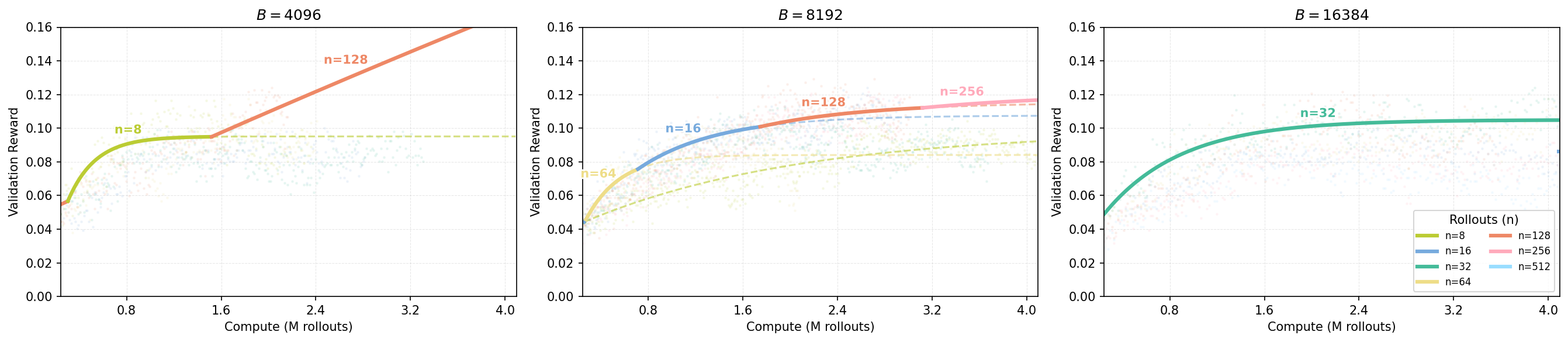
Figure 19: Compute-optimal frontiers on the Hard set under fixed total batch size . Compared to the Easy set, the trends are noisier in the Hard regime. Nevertheless, the qualitative trend remains consistent: as compute increases, the compute-optimal allocation increasingly favors larger parallel rollouts per problem, i.e., larger .
Finally, we report results on the in-domain Extremely Hard subset (pass@128 =0) using both best@4 and worst@4 metrics (Figure 20). We observe a clear coverage–sharpening trade-off: larger is more beneficial for improving best@4 (coverage), while worst@4 (sharpening) is compute-optimally maximized at a moderate (e.g., ). Notably, overly large (e.g., ) can underperform on worst@4 despite achieving better coverage, suggesting that the compute-optimal choice of on extremely hard problems typically lies in an intermediate regime that balances exploration and consistency.
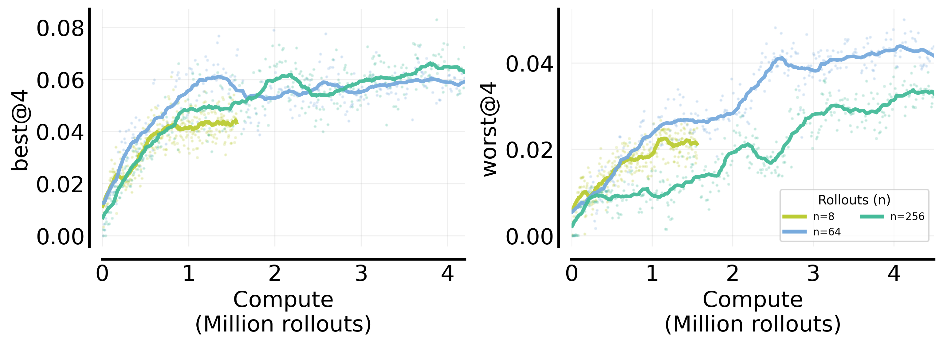
Figure 20: Compute-optimal frontiers on the in-domain Extremely Hard subset (pass@128 =0), evaluated with best@4 (left) and worst@4 (right). Larger improves best@4 at higher compute, whereas worst@4 is maximized by a moderate , highlighting a strong coverage–sharpening trade-off in the extremely hard regime.
B. Generalization to OOD tasks
In the main text, we prioritize in-domain validation results to minimize the influence of train-test distribution shifts, thereby allowing for a cleaner analysis of compute allocation scaling. In reality, practical post-training workflows require models to generalize to unseen distributions like downstream tasks. We examine whether the benefits of increasing parallel rollouts () extend to out-of-domain (OOD) downstream tasks. As illustrated in Figure 21, we observe that larger values of lead to higher performance on AIME24.
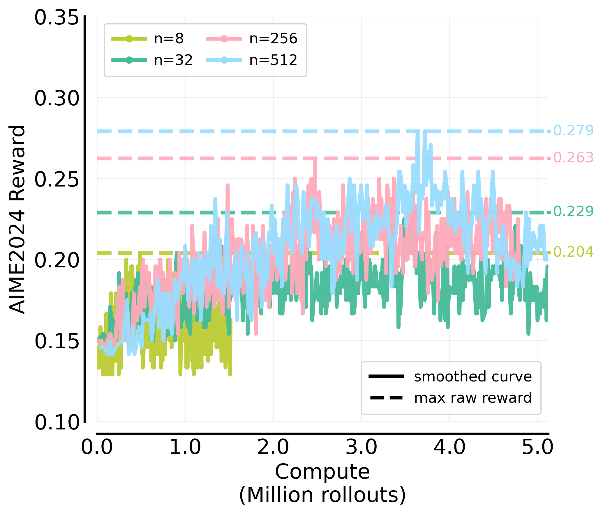
Figure 21: AIME 24 scores trained with varying parallel rollouts () under a fixed problem batch size ().
C. Effects of baseline estimation variance
We discuss in the main content how and why larger could outperform small at high compute regime from exploration and optimization perspective. Another theoretical advantage of larger in the GRPO algorithm is that it provides a more robust estimator for the baseline (group average reward), thereby reducing the variance of the advantage estimates. To isolate the performance gain attributed specifically to precise baseline estimation versus simply training on more data, we conducted an ablation study with a fixed problem batch size of (). We compared three settings:
- Large
- Small
- Decoupled: small for policy update and large for baseline estimation. We generate 256 rollouts to compute high-precision advantage estimates, but randomly subsample only 64 rollouts to compute the policy gradient update.
We observe a performance (1) > (3) > (2).
- (3) > (2) confirms that a lower-variance baseline estimator contributes to the gains.
- The standard (1) run still outperforms the (3) setting, suggesting that while baseline precision matters, the primary benefit of scaling comes from the broader exploration.
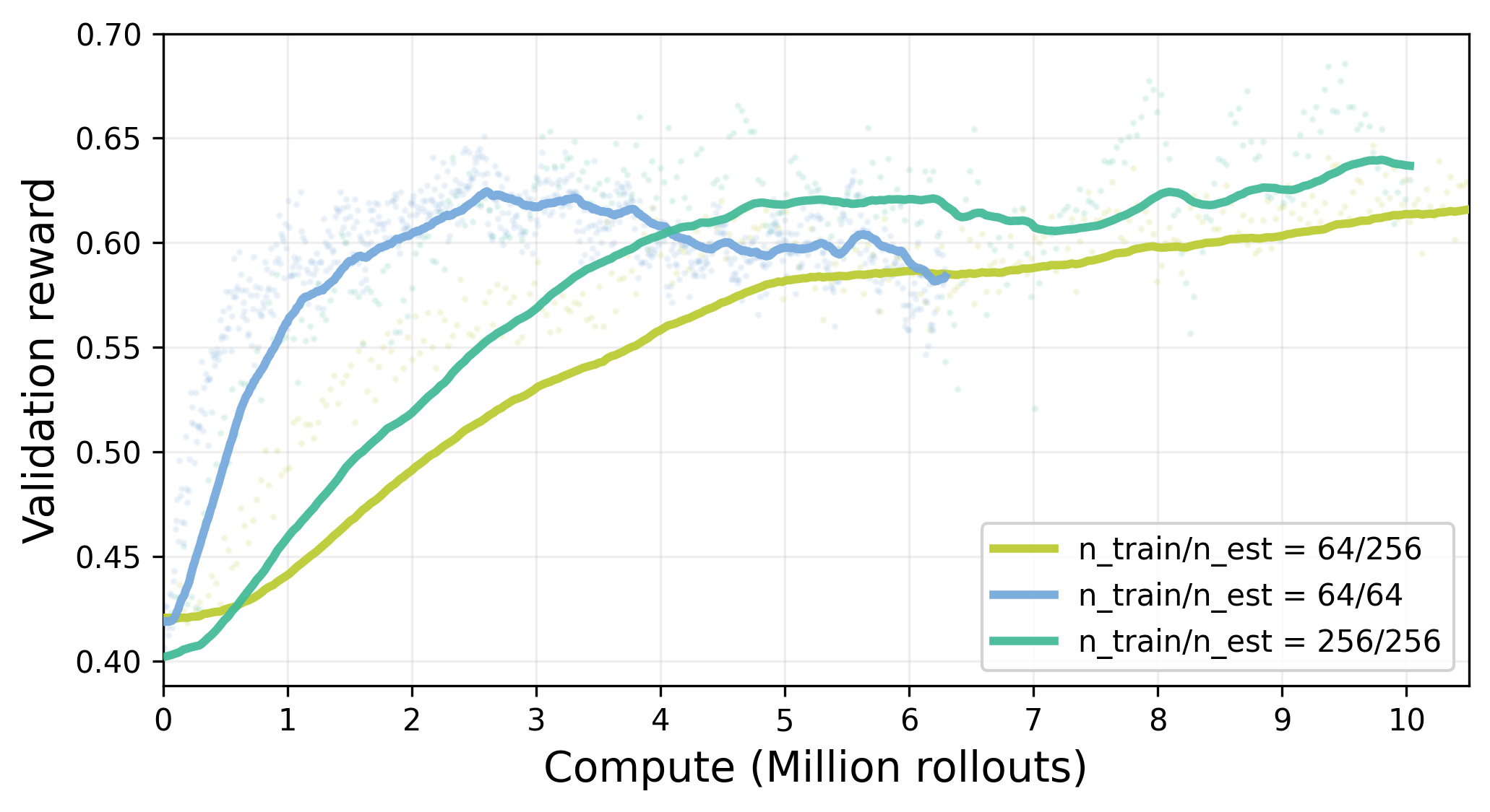
Figure 22: Effects of baseline estimation variance. Validation reward vs. compute (million rollouts) under a fixed problem batch size , comparing three GRPO settings: (i) large group size , (ii) small group size , and (iii) decoupled baseline estimation (estimate baseline from 256 rollouts but sample 64 from them for the policy-gradient update).
We observe consistent ordering (1) > (3) > (2), showing that lower-variance baseline estimation improves performance ((3) > (2)), while the full run remains best, indicating the dominant gains from scaling come from broader exploration beyond baseline precision.
D. Compute metrics #rollouts vs. #tokens
To verify that our compute–optimal scaling is not an artifact of how we measure compute, we repeat the same fit using another unit: total generated tokens. As shown in Figure 23, both parameterizations lead to an almost identical sigmoid trend. This suggests that, for our training setup, using rollouts or tokens as the compute proxy makes little practical difference. The two views are largely related by a near-constant conversion factor governed by the average response length.
One noticeable difference is that the fitted slope parameter is not exactly the same across the two plots. This is expected: controls how sharply transitions as compute increases, and its numerical value depends on the units of . In experiments, we observe a positive correlation between the model’s response length and validation rewards. For instance, models at the high-compute frontier tend to have longer response lengths. Since token-based compute accounts for response length, the value is smaller, indicating a shallower slope in scaling relative to compute. Therefore, the change in mainly reflects how response length modulates the mapping between rollouts and tokens, rather than a fundamental discrepancy in the underlying scaling behavior. Nonetheless, the overall scaling trend remains consistent.
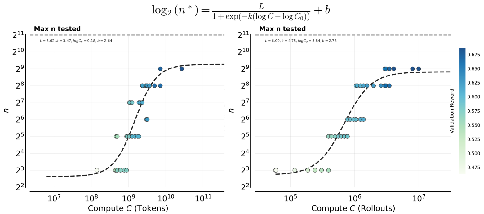
Figure 23: scaling is consistent under token-based vs. rollout-based compute. We fit sigmoid curves for as a function of compute , using either total generated tokens (left) or total rollouts (right). Both choices produce the same qualitative scaling curve—rapid growth followed by saturation—indicating that the compute-optimal trend is robust to the compute definition.
Citation
Please cite this work by:
@misc{Cheng2026isocompute,
author={Cheng, Zhoujun* and Xie, Yutao* and Qu, Yuxiao* and Setlur, Amrith* and Hao, Shibo and Pimpalkhute, Varad and Liang, Tongtong and Yao, Feng and Liu, Hector and Xing, Eric and Smith, Virginia and Salakhutdinov, Ruslan and Hu, Zhiting and Killian, Taylor and Kumar, Aviral},
title={IsoCompute Playbook: Optimally Scaling Sampling Compute for RL Training of LLMs},
howpublished={url{https://compute-optimal-rl-llm-scaling.github.io/}},
year={2026},
}